My first simulation: sky models and Measurement Sets

This first simulation is (hopefully) about as simple as they get. We'll take a sky model, an empty Measurement Set (MS), use MeqTrees to fill the MS with model visibilities and then make an image.

Both the Tigger format sky model and the Measurement Set are attached in the data products below. You'll have to tar -xzvf the MS for it to become useful.

The u,v,w points, the time slots and the frequency setup of the observations you wish to simulate are defined by the Measurement Set, as is the pointing centre. In this case the MS is a 1445 MHz KAT-7 observation spanning 12 hours, with 60 seconds of integration time per visibilty point. There's a single 16 MHz channel and the pointing centre is RA = 19h 15m 53.304s, Dec = -74d39m37.90s.

The sky model is a set of sources drawn from the SUMSS covering approximately the field of view of the KAT-7 instrument. The survey from which they are drawn was conducted at 843 MHz so the sources have had their fluxes extrapolated to what they would be at 1445 MHz assuming a spectral index of 0.7.

Recall that calibration of radio interferometer data involves the generation of a model visibility set for comparison to the measured values. The Radio Interferometer Measurement Equation (RIME) is generally invoked to predict model visibilities based on assumptions about the sky and the instrument. A numerical solver is then employed to minimise the difference between the observed and model values by tuning solvable parameters within the RIME. Typically these parameters consist of a single complex gain term, per feed, per antenna, that is assumed to be a function of both time and frequency. These best fitting gain terms can then be applied to the observed data in order to remove the gain drifts imposed by instrumental and atmospheric effects. This is basically why any calibration package worth its salt will offer simulation capability: the prediction stage is an essential part of calibration, so if you're calibrating data you need the machinery for simulation.

MeqTrees comes bundled with a simulation framework known as Siamese, which lives in the Cattery folder. Load up the meqbrowser, attach to a server, select "Load TDL script" from the TDL menu, navigate to the Siamese folder and load turbo-sim.py.

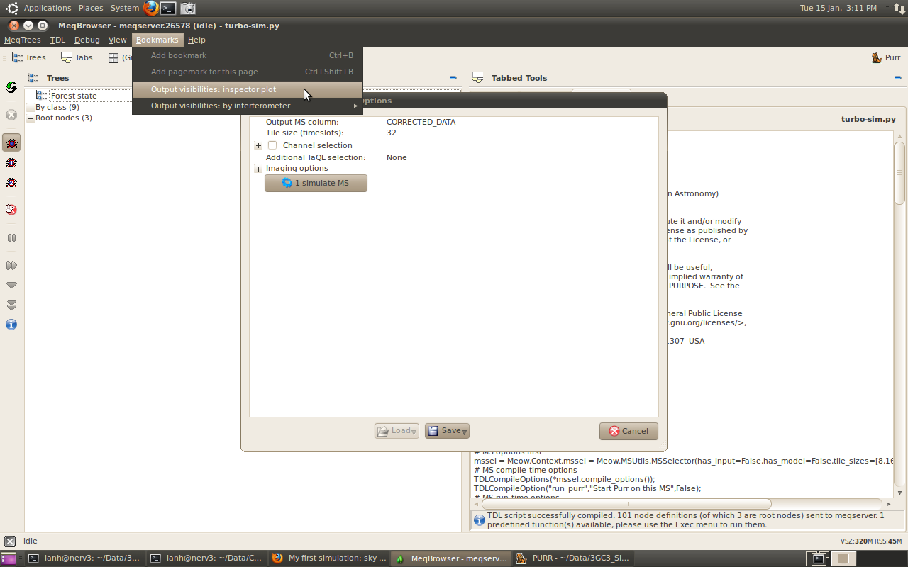
Executing anything via the meqbrowser is generally a two-stage process. The first stage involves setting "compile time" parameters (accesible with the "TDL Options" button in the bar) which determine what you want to do, the second stage asks for "run time" parameters (accessible via the "TDL Exec" button) which determine how you want to do it. In between these two processes you have the opportunity to open bookmarks, which let you visualise various things as the simulation or calibration progresses.

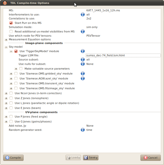
Once turbo-sim.py has loaded you should be presented with a screen full of compile time options. You can expand or collapse any of the subsets of hierarchical options by clicking the "+" or "-" signs. As you can see there are a lot to choose from, and for this simulation we'll be ignoring most of them.

The compile time options screen shot below shows how to set up this first simulation. We're basically pointing the script at our Measurement Set (KAT7_1445_1x16_12h.ms), and telling it we're using a Tigger format sky model, and which one we want to use (sumss_dec-74_field.lsm.html). The rest of the options remain unchecked. Another important switch however is the "Simulation mode: sim only" option. This just means the visibilities generated by this simulation will overwrite whatever is in the MS. You can also add and subtract to existing visibilities which is useful and will be used in other simulations. We're using all interferometers (synonymous with baselines), all correlations (polarization products) and all sources in the sky model.

"Start Purr on this MS" is also checked. I'm not going into the details of it but Purr is a nice bit of bookkeeping software. I obviously wanted to activiate it in this case as I'm using it to make the web page you're currently reading.

Once this is all set up click "Compile" and MeqTrees will build a simulation tree.

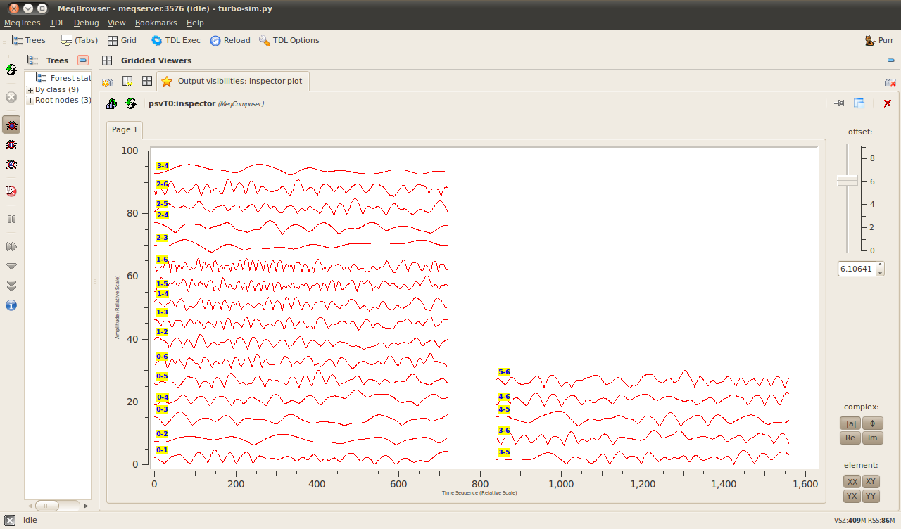
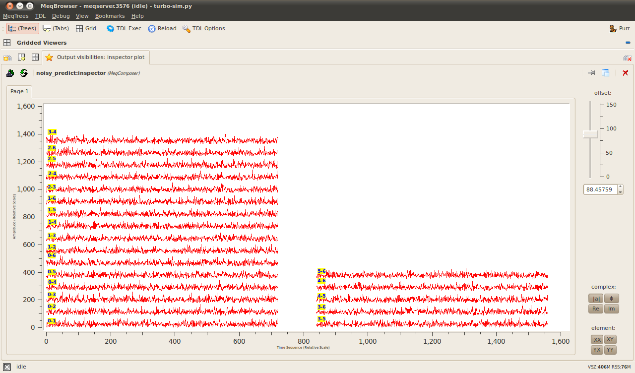
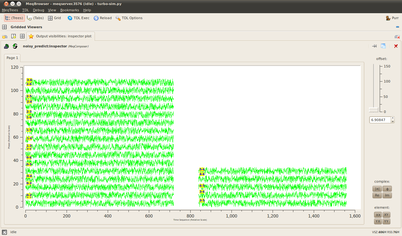
At this point you can add a bookmark. These allow you to visualise the values of arbitrary nodes in the tree. Some pre-defined ones are provided by turbo-sim.py. Try visualising the visibilities as they get generated by selecting the appropriate item in the "Bookmarks" menu as per the screenshow below. Screenshots of the amplitudes (red) and phases (green) of the visibilities as a function of time, per baseline are attached below.

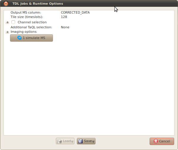
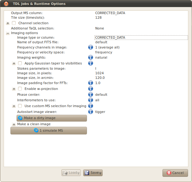
The runtime options for this script are pretty simple, as shown in the screenshot below. The important ones for now are the "Output MS column" which tells MeqTrees where to put the simulated data in the MS table structure. The "Tile size (timeslots)" option determines the size of the data chunks that are processed. Generally, the higher this is the less time it will take to process your simulation, and how high you can set it generally depends on how expensive your computer was. It won't make much difference here though as this is such a small simulation. Ignore "Imaging options" for now, we'll get on to those in the next section.

Once you're ready click the "1 simulate MS" and you should see a bunch of simulated visibilities spew forth into the viewer window.

Visibility plots are all well and good, but nothing lifts your mood like a radio image, so let's make one.

The turbo-sim.py script (along with many other of the stock MeqTrees scripts) allows us to invoke the CASA-based lwimager directly from the GUI. To do this, click the "TDL Exec" button in the tool bar to bring up the runtime options again, and expand the "Imaging options" submenu.

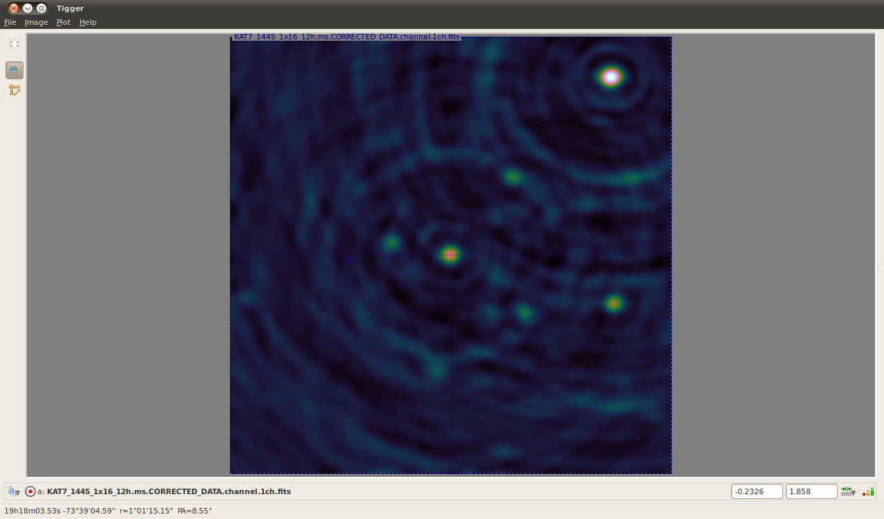
The main thing to get right here is the "Image type or column" option, to make sure we're actually forming an image from the MS table where we just stored our simulated visibilities. MeqTrees usually remembers what you did and will set this option accordingly, but double check it. You can also select "PSF" here to make an image of your point-spread function (aka dirty beam).

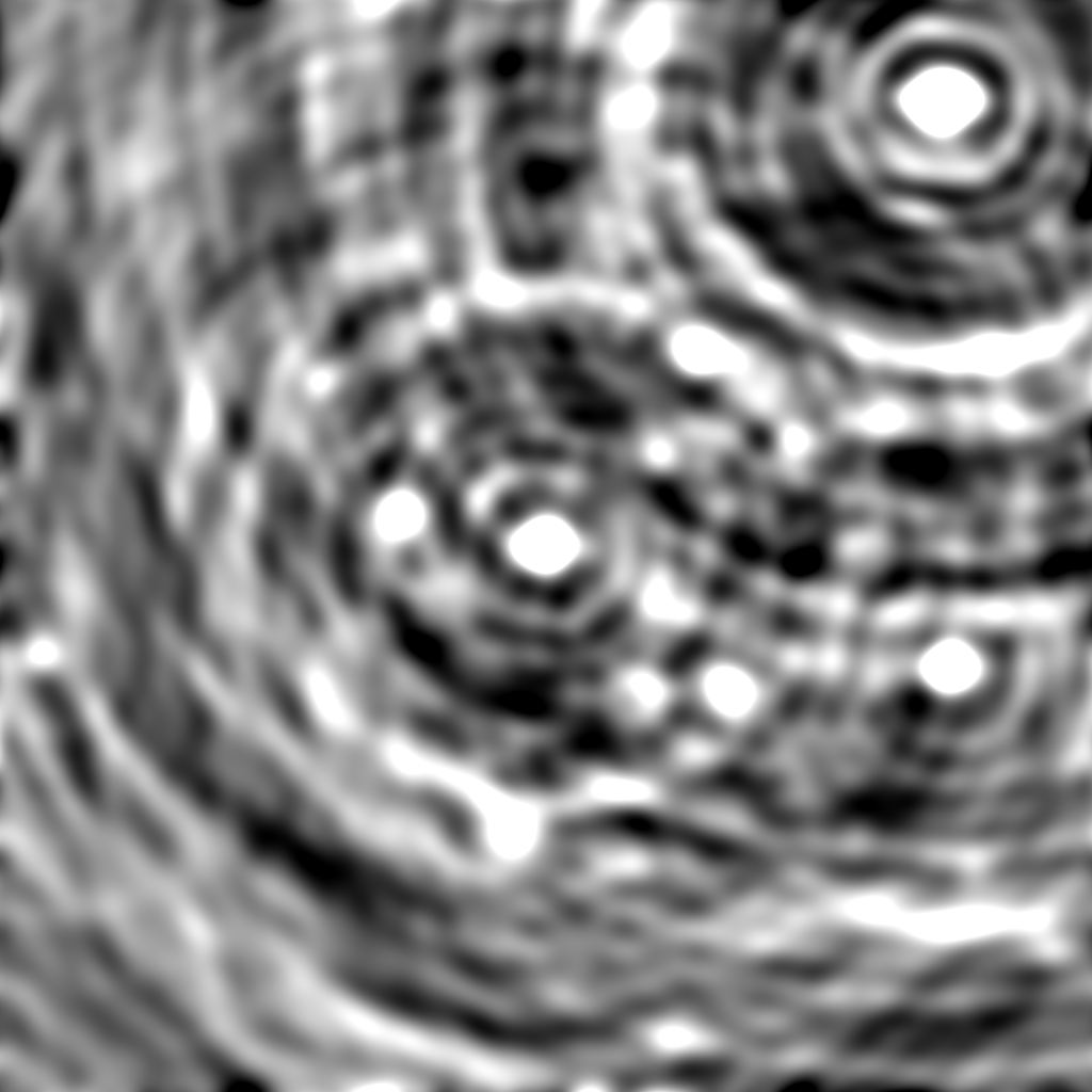
Playing around with these options is encouraged. The setup I used to make the image attached to this entry is presented in the screengrab below. The image is 2 x 2 degrees (1024 x 1024 pixels) and no deconvolution has been performed.

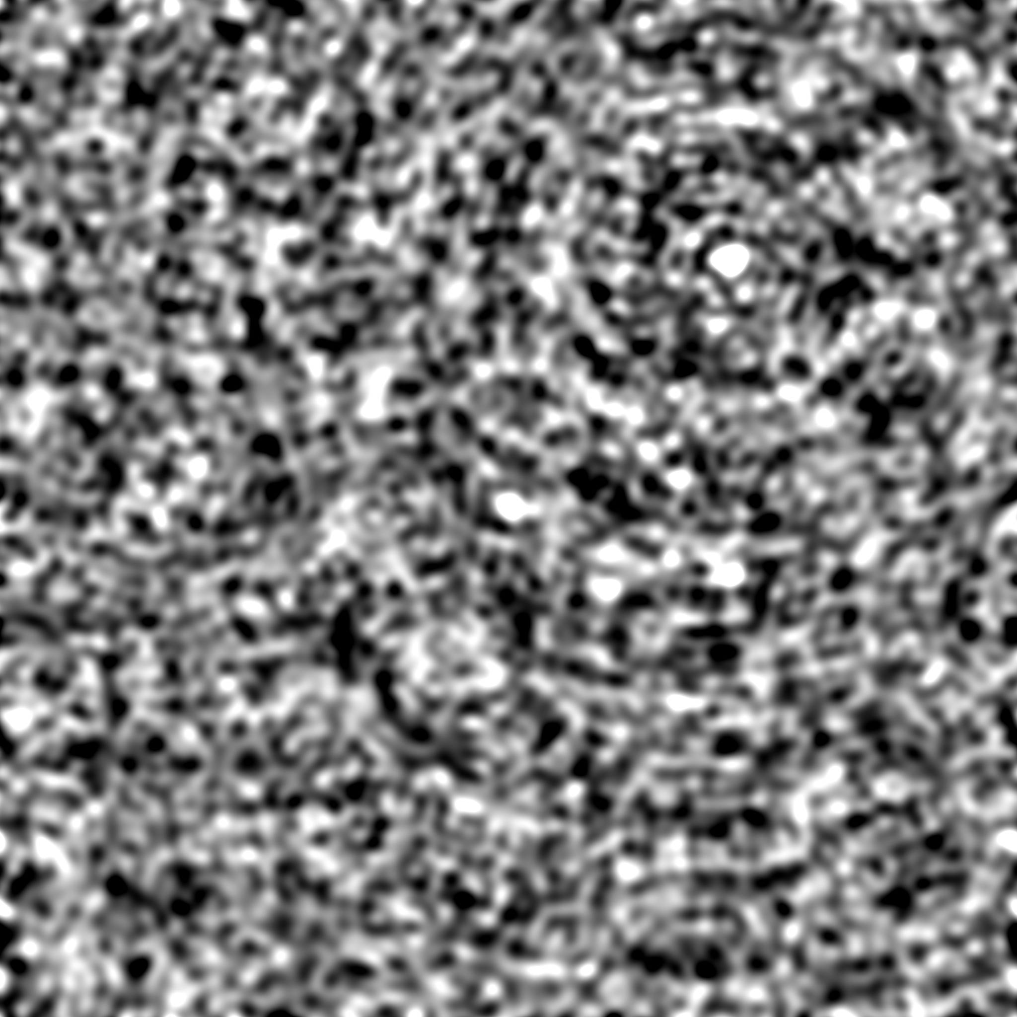
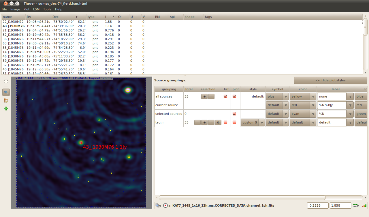
Once the image has been made, and unless the relevant parameter has been changed, the Tigger image viewer will pop up and show you the map, as per the screenshot below. Tigger is not only an image viewer but is also used to manage its own sky model format. Opening summs_dec-74_field.lsm.html via the file menu will allow you to compare the model sky component list to the image (screenshot below). You can see that most of the fainter sources are swamped by the sidelobes of the bright source to the north west. Playing around with the deconvolution ("Make a clean image") options might allow you to see a few more sources...

In the opinion of your humble correspondent there are two reasons for doing simulations. The first is when you are writing a telescope proposal and you wish to convince the time allocation committee that you've at least considered the feasibility of detecting something with their precious telescope time. The second is when you want to investigate the vagaries of radio interferometry and the multitude of subtle mindbending effects that it encompasses.

In the first scenario the inclusion of thermal noise is absolutely essential. In the second scenario it may or may not be called for.

Since the set of simulations to which this particular example belongs are very much of the second kind, thermal noise will largely be ignored.

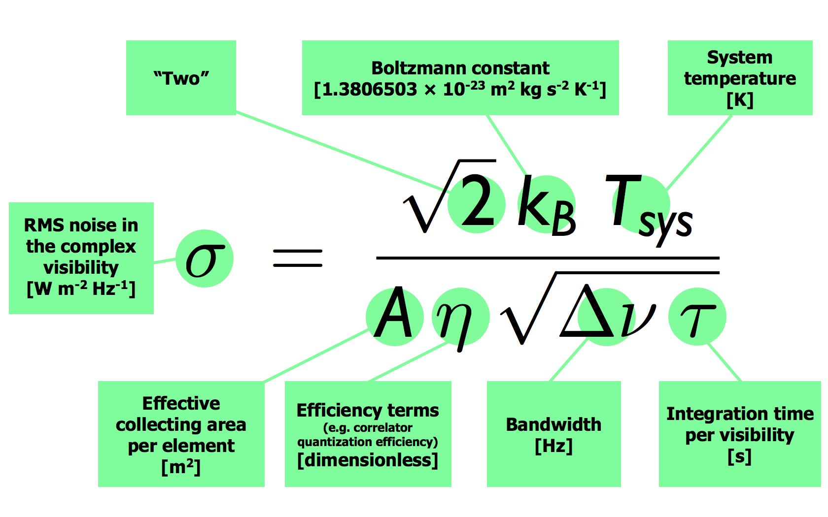
You can add noise to the simulation using the turbo-sim.py script; note that the "Add noise, Jy" option in the compile-time options of turbo-sim.py is the noise per visibility measurement, not the desired noise in your image. You can evaluate what value you should enter here by plugging a bunch of sensible assumptions about your instrument and a couple of parameters from your observational setup into Eq. 6.50 in "Interferometry and Synthesis in Radio Astronomy", Thompson, Moran and Swenson (2nd. Ed.) -- see the attachment below.

We will perform a simulation here with thermal noise to illustrate a very important point about radio interferometry.

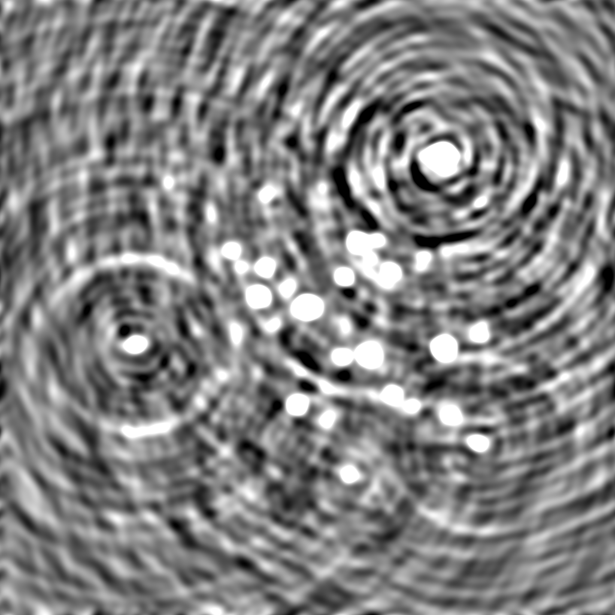
If you evaluate the equation below for a typical observation then you might find the value is surprisingly high. Consider the set of Compile time options that have been attached below, (along with the TDL configuration). As you can see I've added (apropos of absolutely no rigourous calculation to arrive at this value) 20 Janskys of noise to the simulation.

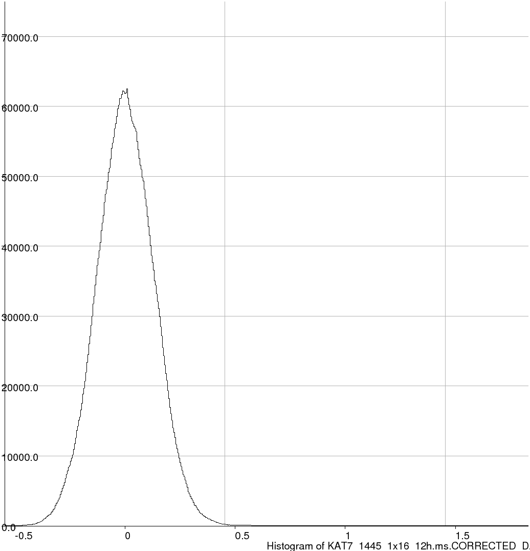
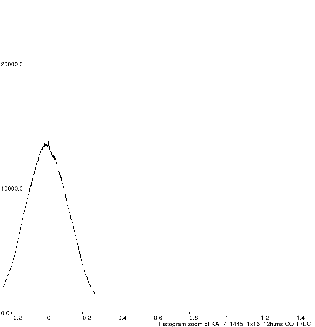
If I compile this simulation, open a bookmark to take a look at the output visibilities, and then run the simulation from the TDL Exec menu, I can see that the amplitudes (red plot, below) and phases (green plot, below) both resemble noise. Contrast these to the plots generated in the previous noise-free section. The amplitudes and phases are nice smooth functions in time; the visibility function is modulated by the superposition of the sinusoidal fringe contributions from each source in the field.

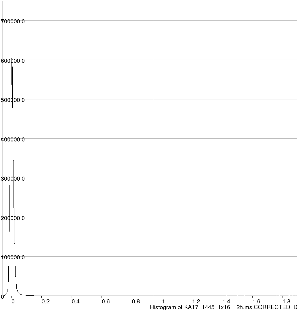
Yet if I pop up the TDL Exec options once again and make a dirty image (attached below) I can still see a few sources. The brightest source in this simulation is 1.88 Jy. Yet it is sitting there (at a signal to noise ratio of about 14, no less) in the presence of 20 Jy rms of noise.

You may be asking yourself the most important question in science at this point.

We've already touched on the reason for this being possible: the noise we added is applied to the complex visibility and not the image. The pixels in the image are the result of an averaging process that can take in huge numbers of indepedent visibility measurements. Any individual visibility measurement may be very noisy but the contribution of the sky signal to the visibility function is always there, and with many measurements being combined together to form the final image the noise averages out. It's a classic 1/sqrt(N) scenario. Fortunately for radio astronomers (although not so fortunate for the person who has to supply our hard disks), the value of N is frequently huge.

This large number of independent data points (remember that your map pixels are not independent measurements, but your visibility data are) is also highly advantageous for calibration: typically we have a lot more measurements than we have unknowns when solving for calibration solutions.