Corrupting and calibrating complex gain solutions

As mentioned in the previous "Simulations 101" section, the usual ("2GC") approach to calibration involves determining corrections for the complex gains for each receiver in the array (generally for each pair of feeds at each element in the array). The gains of the instrument drift over the course of an observation generally due to the electronics and the atmosphere. These drifts can be solved for if the ideal response of the instrument to the sky is known. The response to a bright point source is a trivial prediction which is why such such sources are often used as phase calibrators in the case where the science target is either unknown or faint. Observations of the target are alternated with visits to a strong point source on a switching timescale that is short enough to track the expected drifts in the complex gains.

(The phase variations induced by the troposphere become more severe with increasing frequency, which is why a fast swtiching scheme is often needed at frequencies above ~15 GHz.)

This simulation demonstrates the calibration principle in a very simple way. We'll simulate an observation of a central point source, then fake some gain variations on the observation and examine the difference. Finally we'll solve for these gain drifts and remove them.

We're going to be using the sky model and Measurement Set from Simulations 101 again. This sky model contains a central point source with an intrinsic flux of about a Jansky, the sort of thing that makes an excellent phase calibrator.

Attached once again are the sky model and the MS.

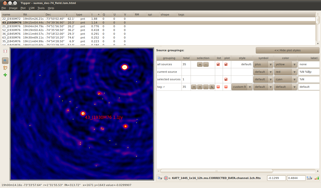
First thing we need to do is make a note of the name of the central point source. If you load the sky model into Tigger and sort by the Stokes-I flux then we want to identify the source with I = 1.14 Jy. If you have a FITS image of this field left over from the previous run then loading this up shows that we have indeed selected the central source -- see the attached screen grab.

It's called 43_J1930M76, so scribble that down somewhere, or leave your Tigger window open, or if you're unlike me and have a functional memory then simply memorize it.

The next thing we're going to do is simulate the visibilities for a sky model consisting only of this source with no instrumental effects and no thermal noise.

Start the meqbrowser, connect to a server and load turbo-sim.py. If you're coming here straight from the previous simulation exercise then Ctrl+1 in the browser should do that last step for you.

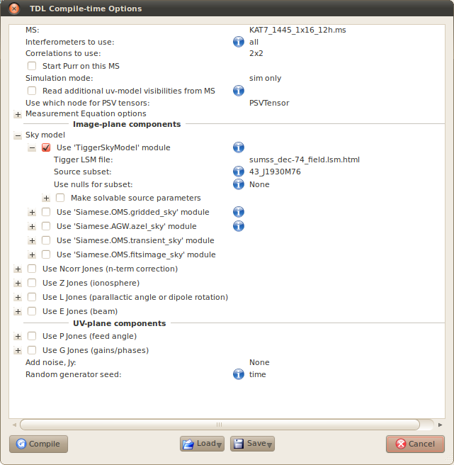
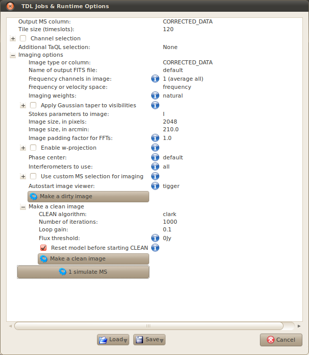
Set up the options as per the screengrab below, or by loading up the attached central-point-source-no-G.tdl.conf file. Note that none of the UV-plane components are activated, and the only image-plane component that we are interested in in the sky model. Specifically, we have put the name of the central source that we identified earlier in the 'Source subset' field.

Compile the script and when the run time options appear, write the visibilities to the CORRECTED_DATA column.

Once the simulation has completed, click the 'TDL Exec' button and make a clean image with some sensible parameters. We now have a reference 'ideal' image for comparison to what is to follow.

Note that we'll be overwriting the CORRECTED_DATA column in the next section and making an image of it. Since that process will overwrite the FITS file we just made if we apply the default file names, you might want to rename or duplicate the

KAT7_1445_1x16_12h.ms.CORRECTED_DATA.channel.1ch.restored.fits

file that just got created.

We'll now repeat the above simulation, but corrupt the receive gains a bit to see the effect this has on our image quality.

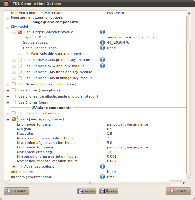
Click 'TDL Options' to bring up the compile-time options again. The only change we're making here is to activate the 'Use G-Jones (gains/phases)' option in the UV-plane components section. There are a few toy error models that you can play around with here. You are encouraged to experiment, as always!

The example I've made here (see attached screenshot) is to apply a periodically varying error to the gain and phase components. This applies a sinusoidal wobble to these parameters for each antenna with the values swinging between the min and max levels. The period is randomized between the specified min and max values, resulting in different drift rates for each element in the array.

Once you're happy with your options, click 'Compile'.

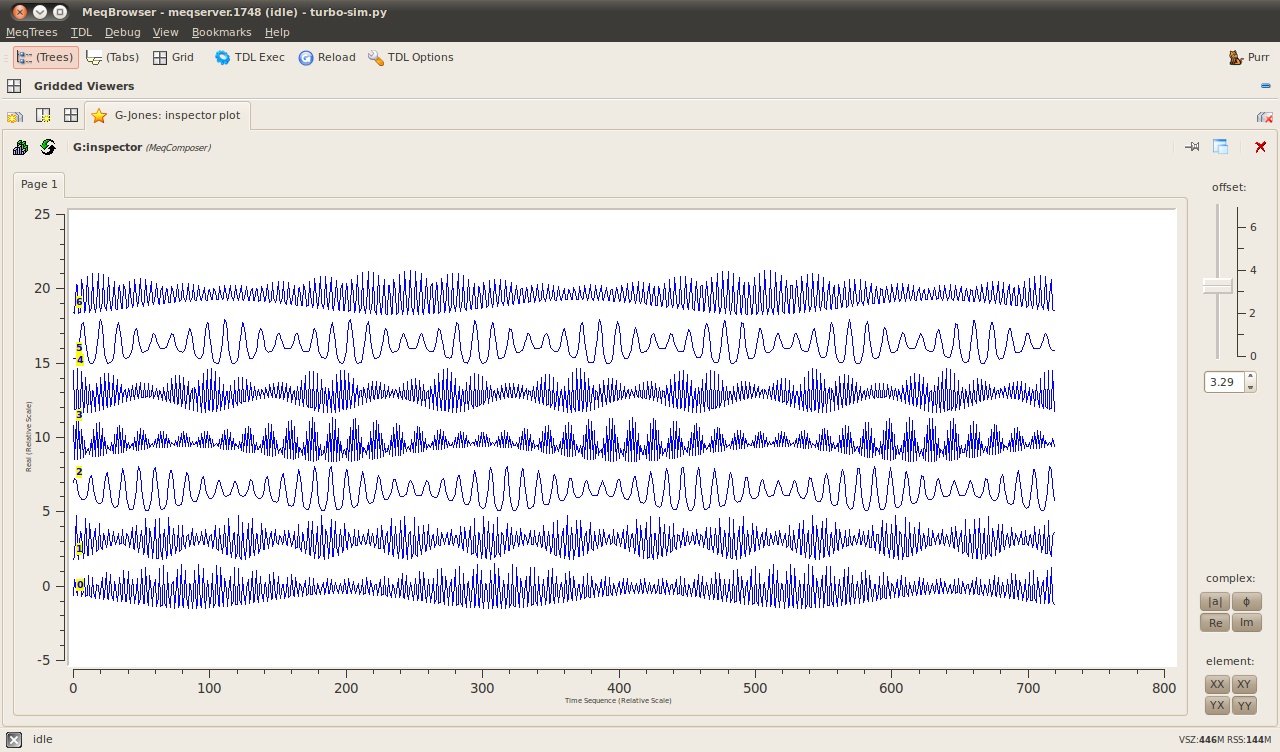
You can open a bookmark at this point to see the gain variations that are applied to each station: 'G-Jones: inspector plot'. After this, check that we're writing to the CORRECTED_DATA column and hit '1 simulate MS' from the run-time menu.

The screenshot of the browser below shows the Real part of the gain corruptions for each of the seven antennas in the array for the YY polarization. You can flip between the complex products and the polarization products in the viewer using the buttons in the lower right.

Now let's make another cleaned image. In the spirit of all-other-things-being-equal, we need to use the same parameters as in the previous section, which should have been remembered by the browser anyway.

The TDL configuration file for the above is attached below (central-point-source-G.tdl.conf).

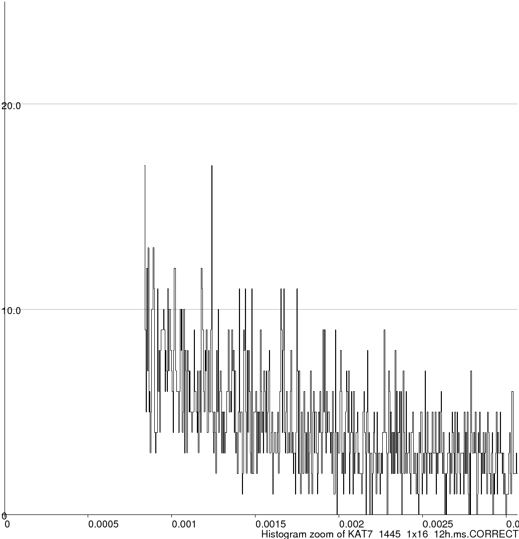
The easiest way to see this is to look at the statistics of the two cleaned images we made. The stats dervided by Purr when it attaches FITS files to a log such as this one will suffice, and these are available in the data products of the previous two sections.

The 'data range', the 'clip range' and the image thumbnails can provide a pretty decent picture of what's happened.

The data range values simply list the minimum and maximum values of the image in map units (Jy/beam, typically). For the first uncorrupted case the data range has an upper value equal to the intrinsic flux of the source. The feature in this map accurately reproduces its true flux. Compare this to the upper data range value in the second image. This peaks out at 0.095 Jy/beam, i.e. the source has been attenuated to below 10% of its true value!

Consider the screengrab of the Real part of the complex gain corruptions above. Although the sky is constant, the differing gain drifts in each station mean that the each element in the array sees an artificially attenuated (or amplified) signal that drifts in time. Remember the noise section in 'Simulations 101': making a map averages the many visibility measurements, and in this case we recover some 'average' flux that is way off the true value.

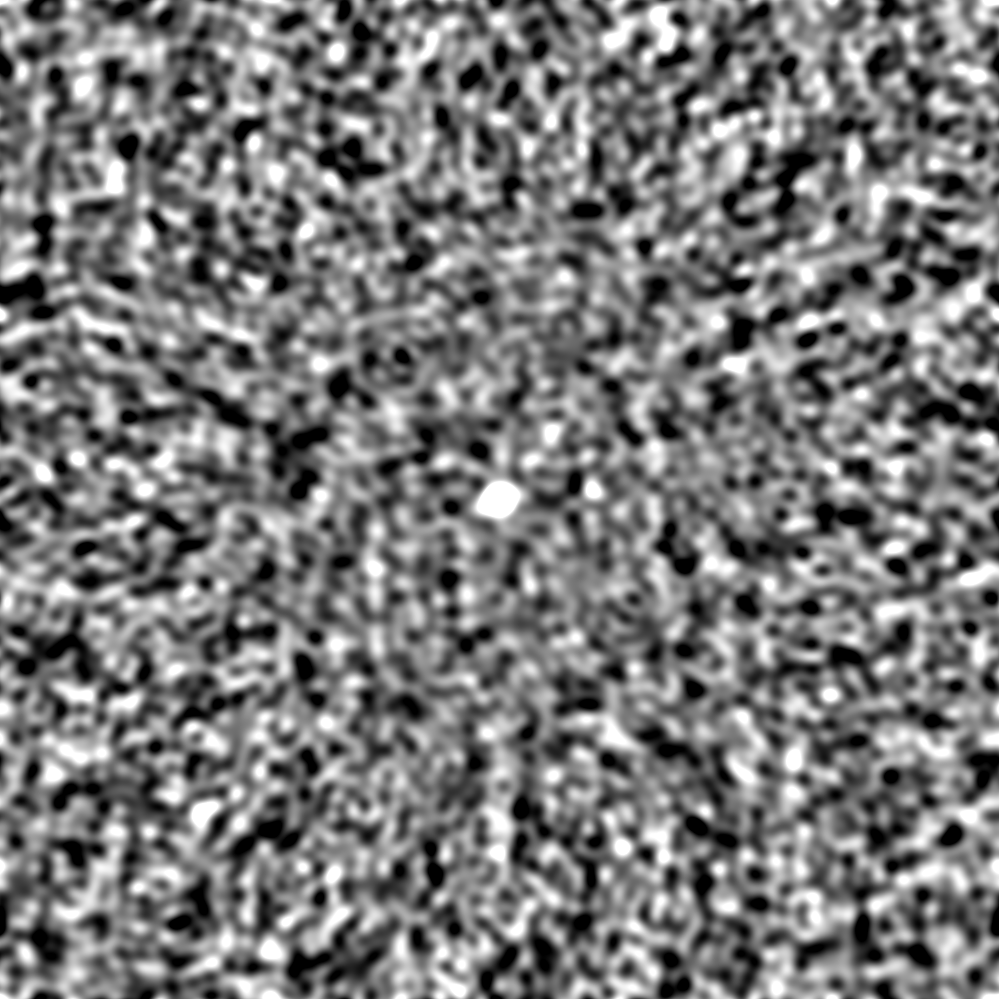
Remember also that we have attempted to deconvolve this source, albeit not very carefully, just 1000 blind iterations of clean over the whole field. Still, this should have been enough to remove the PSF sidelobes from the regions away from the source. This is where the clip range values and the image thumbnails demonstrate the other horrid effect of varying G-terms. The clip range shows the upper and lower pixel values that have been applied to render the thumbnail image.

For the first simulation with no gain corruptions the clip range spans 0.8 mJy to 3 mJy, and no background structure is visible. If you examine your FITS image here in Tigger you can see that the background structure is extremely low-level; it essentially results from the deconvolution imperfections. For the second, corrupted simulation the range is -8.9 mJy to 10 mJy. This range obviously covers much brighter emission and as can be seen from the thumbnail there is plenty of it. This emission is a fundamental 'noise' limit in this simulation. Deconvolution can't take care of it, only calibration can.

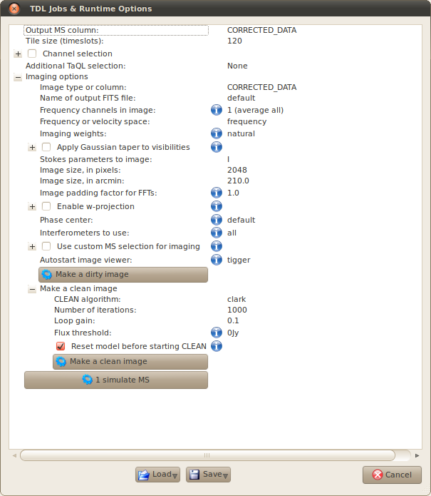
Before we proceed, let's repeat the corrupted simulation above, but this time write the results to the DATA column. When you get genuine radio telescope data from an observatory this is where your raw visibility measurements live. If you haven't changed anything from the last run, then just click TDL Exec, change the 'Output MS column' to 'custom', enter 'DATA' in the relevant box and re-simulate the visibilities.

Once this is done, let's use a calibration script to try to get rid of the corruptions we've just put in. As well as the 'Siamese' simulation framework, there are some example calibration scripts in the Cattery under the 'Calico' folder.

Close and restart the meqbrowser, select 'Load TDL script' from the TDL menu, and open calico-wsrt-tens.py. As with the simulation script, this takes a Measurement Set and a sky model and constructs a measurement equation with various image plane and uv-plane terms in it. The difference here is that the Measurement Equation contains solvable parameters, and instead of simply predicting data and writing it to the MS, it predicts data and compares this to the existing data the that MS contains. A numerical solver minimises the difference between the observed and the predicted by tuning the solvable parameters.

The Measurement Equation paradigm offers ridiculous amounts of flexibility, as partially evidenced by the daunting amount of compile time options in that popped up when the script laoded, but all we'll be solving for here are the G-Jones terms, i.e. a single solvable complex gain term for each element of the array. Most of the options can be ignored for now.

Point the script at the Measurement Set that contains the simulated visibilities, and as before in the skymodel section select the "Use 'TiggerSkyModel' module" and load sumss_dec-74_field.lsm.html. Our assumed sky model here is the central point source only, i.e. source 43_J1930M76.

So far, so simulation.

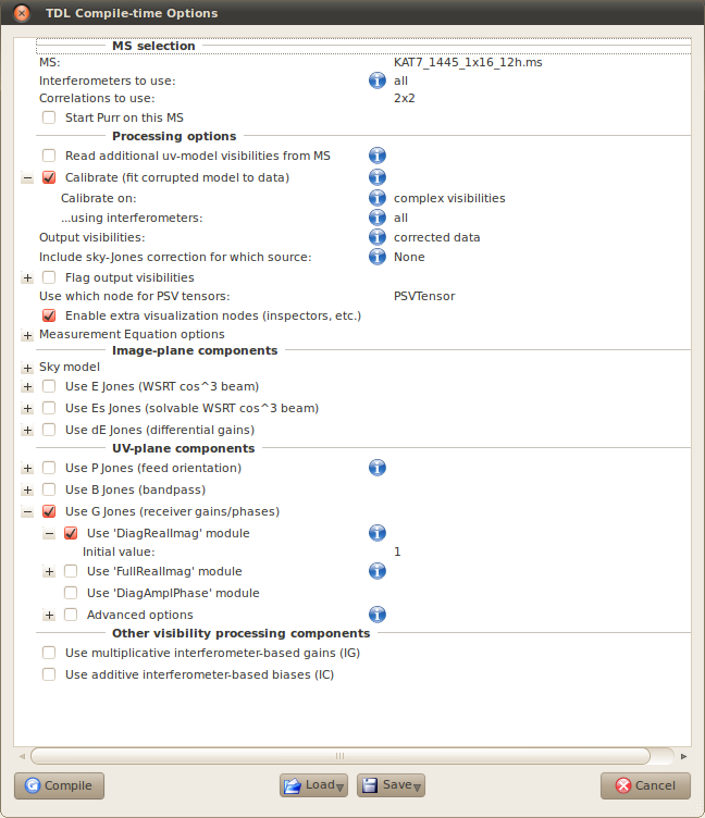
The first new part here is the 'Processing options' section. Check 'Calibrate (fit corrupted model to data)', we want to 'Calibrate on:' 'complex visibilities', and set the 'Output visibilities:' to 'corrected data'. Check also 'Enable extra visualization nodes (inspectors etc.)' as bookmarks are always useful and we'll want some in a minute.

As mentioned above we're just solving for the G-Jones terms here, so check 'Use G Jones (receiver gains/phases)' ad select "Use 'DiagRealImag' module". This just sets up a 2x2 Jones matrix for each antenna with solvable terms on the diagonal (XX/YY).

Click 'Compile' and the meqbrowser will build your calibration tree.

The runtime options should pop up now, but before we look at those let's open a bookmark. If you only open one bookmark this session let's make it the 'G Jones: inspector plot' one.

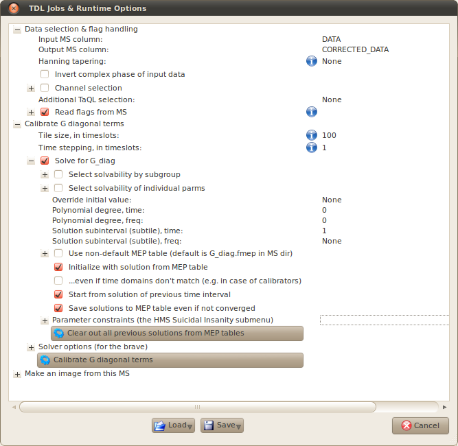
There are a few more options in the run time menu than we are used to with the simulation script. An important pair to get right is the 'Input MS column' and 'Output MS column' in the 'Data selection & flag handling' menu. Expand this and check that the former says DATA and the latter CORRECTED_DATA. This ensures we're solving for the gain terms in our parametrized Measurement Equation by comparing them to the correct 'observations', i.e. the results of our corrupted simulation. The observed DATA will be divided by the best fitting gain terms at the end of the calibration, and the resulting visibilities written to CORRECTED_DATA for imaging or further processing. The calibration process is (and should be) non-destructive, preserving our original measurements at all times. (That doesn't mean you don't need a backup, though!)

The other thing I've checked here is the 'Read flags from MS' option. In a real observation you don't want to be solving for data that you've flagged as RFI for example. When I made this simulated KAT-7 MS I included flagging for antenna elevations below a certain threshold, although to be honest I'm not sure this threshold is ever reached at this Declination. I suppose I should look at the flag columns in the MS...

Moving onwards: expand the 'Calibrate G diagonal terms' submenu. Most of these values can be left at their defaults. The important one is the 'Tile size, in timeslots'. The timeslot in this case is whatever the native time resolution of the MS is (I believe it's 30 seconds, but you can collect bonus points by having a look at the EXPOSURE column in the main table if you're curious). Anyway, what setting this parameter does is determine how much of the data MeqTrees reads in at a time. For a job of this size on a decent spec machine you can probably set this pretty high. I've set it to 100 here. The G Jones option in this calibration script by default reads in all frequency channels, but our simulation only has one so this is not an issue. The 'Time stepping, in timeslots' option remains at 1 as we want to calibrate every time slot.

Ensure the 'Solve for G_diag' option is checked. There are some more values here that we need to ensure are correct, that offer additional flexibility in how each of the tiles we extract for calibration are processed. As mentioned before we want to solve for every time slot here, so make sure the 'Solution subinterval (subtile), time' option is set to 1. The frequency option is not relevant.

The gain solutions themselves are stored in something called a MEP table (I believe this stands for Measurement Equation Parm). Some slightly more advanced calibration scenarios required multiple passes, or additional solvable terms in the Measurement Equation, and storing the solutions from previous passes prevents them having to be recomputed each time. MeqTrees stores these by default inside the MS (G_diag.fmep), and as you can see from the options here it will take any existing table (either specified or default) as the starting point for the calibration. If something goes wrong and you need to repeat the calibration it's important to remember this, and if necessary make use of the 'Clear out all previous solutions from MEP tables' button!

The 'Solver options' submenu can be ignored for now, and the 'Parameter constraints' submenu can hopefully be ignored for ever.

Once you're happy with your parameters and bookmarks, click the 'Calibrate G diagonal terms' button and watch the plots roll in.

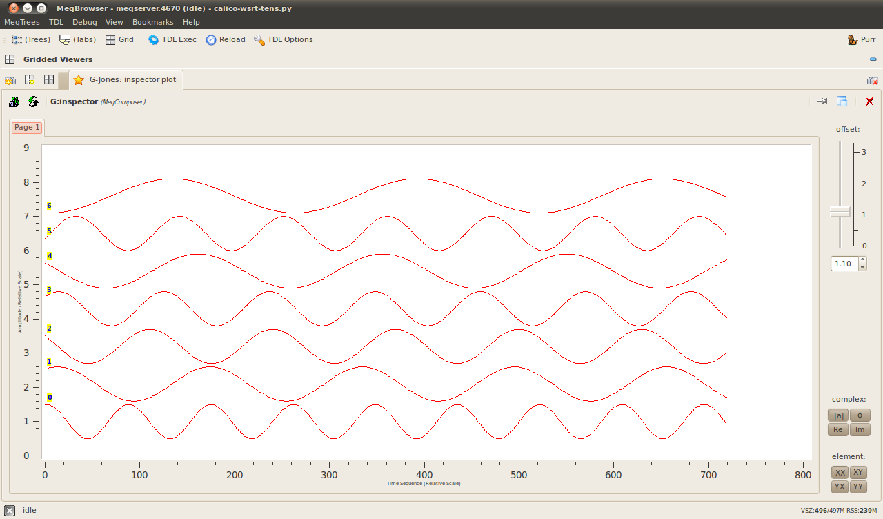
The derived gain solutions (G-Jones) as traced by the bookmarks window are shown below. The sinusoidal drifts that we applied to each antenna are clearly captured by the solver.

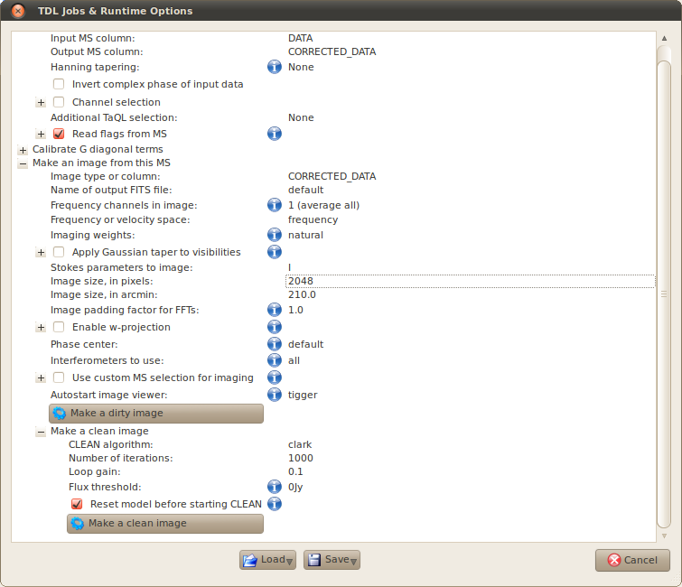
Those gain solutions look promising, so let's see how good the calibrated map looks. Click the TDL Exec button again and make a cleaned image in the same manner as above (options grabbed below).

As you can see we've identified and corrected the gain drifts. This is a simplistic example, and the real world is never this well-behaved, but the methods we have covered here represent the fundamentals of all calibration.

You are encouraged to repeat the calibration, varying some options. Some things to try:

i) Vary the 'Solution subinterval (subtile), time' option in the 'Solve for G_diag' submenu. This averages up the data and then performs the solution on that product. This is faster than solving for every time slot but is less accurate. How does the solution subinterval affect how well you recover the true sky?

ii) Add some extra sources from the sky model into the calibration. What happens when you calibrate against a sky model that isn't correct? Are your sky models ever truly accurate?

iii) You can get a handle on how well your calibration has gone by asking MeqTrees to produced corrected residuals instead of corrected data at compile time. This is particularly useful for seeing how accurate your assumed sky model is, and for e.g. item (i) above it will naturally tell you at what level the imperfect calibration is going to pervade your map.