What is the primary beam? What is the primary beam?
Logged on 03/02/13 13:55:40
This simulation is designed to illustrate the first order effects of the primary beam. It also introduces a the useful tricks that is making difference images in Tigger.
In radio astronomy you will generally hear people talking about two things that involve the word 'beam'.
i) The dirty beam: this is the point spread function (PSF) of an observation, i.e. when you Fourier transform your visibility measurements to obtain your image of the sky, it it convolved everywhere with the dirty beam pattern. Your image at this stage is known as the dirty image, i.e. it needs cleaning up with a deconvolution algorithm to remove the sidelobes of the dirty beam that are associated with each region of emission from the sky. The shape of this pattern is determined by how filled your aperture is, i.e. how good your uv plane coverage is. The Fourier transform of your uv coverage determines the shape of the dirty beam. Some people (myself included) prefer to refer to the dirty beam simply as the PSF as it (hopefully) avoids confusion with the other type of beam, namely...
ii) The primary beam: to first order the primary beam can be thought of as the sensitivity of your instrument as a function of direction. The receiving elements that make up the array are not uniformly sensitive to incoming radiation from all directions. For example, an array of parabolic dishes has maximum sensitivity in the direction which they are pointing (typically the phase centre), and the sensitivity drops off away from that direction. As a rule of thumb, the half power point in radians, i.e. the angular distance from the phase centre at which an intrinsic 1 Jy source has an apparent flux density of 0.5 Jy is roughly (wavelength / 2D) where D is the diameter of the dish.
Traditionally the primary beam pattern is assumed to be identical for every receptor in the array, with its effects removed from an observation by dividing the final deconvolved image by some assumed average primary beam pattern. The end effect of this is to correct the attenuated source fluxes, although this process also effectively results in increased image noise towards the map edge.
In reality the primary beam pattern is complicated business, and its inevitable presence in all observations can easily become a fly in your delicious bowl of radio astronomy soup. For example, the many sidelobes beyond the central main lobe that make the interferometer sensitive to sources in the far field. Bright sources can be particularly troublesome as we will see in a later simulation.
The assumption that beam patterns are the same for each receptor is also not a valid one. It is obviously the case for heterogeneous arrays such as e-MERLIN or some VLBI networks, and less obviously for aperture arrays such as LOFAR. However for observatories such as the VLA that ostensibly have identical elements making up the array, subtle effects like the finite pointing accuracy of the antennas result in each station having a slightly different effective primary beam.
Although the problem of bright sources limiting the dynamic range of an image are long familiar, subtle beam effects such as pointing error have only hitherto reared their head for the deepest observations. If your targets are faint enough though, these can prove limiting. But lest we forget: all these radio telescopes that are getting built or getting upgrades are expected to be able to routinely detect the faint radio sky.
Anyway, let's back up a little bit...
The simplest (and therefore friendliest) primary beamLogged on 03/02/13 21:13:15
There might be a case for arguing that the ideal primary beam pattern is an omnidirectional one, i.e. your instrument sees the whole sky. In fact I'd encourage the astronomers, the software people and the hardware people to get into their respective camps on this matter and have a big fight about it.
Before that happens though, let's just introduce the sort of primary beam you get in an ideal world. It's the simplest direction dependent effect: the gain of your instrument drops as you move away from the phase centre, eventually it drops to nothing and stays there until the horizon. It doesn't change with time and it only changes with frequency in a way you don't mind.
Ladies and gentlemen: the WSRT cos-cubed beam.
What we'll do now is take the KAT-7 simulation that has appeared previously with the sky model derived from SUMSS. We'll quickly repeat the initial 'Simulations 101' setup for comparison. Then we'll repeat this with the analytic cos-cubed model for the primary beam and compare the results.
Simulations 101 reduxLogged on 03/02/13 21:15:50
Here we'll just re-do our initial sim for a comparison. I'll rush through this here so revisit the relevant Purr log if you want the details.
It's basically:
1) load turbo-sim.py
2) find your KAT7_1445_1x16_12h.ms in the compile time options
3) point your Tigger LSM file option to sumss_dec-74_field.lsm.html
4) make sure everything else is unchecked
5) write to the CORRECTED_DATA column during run-time
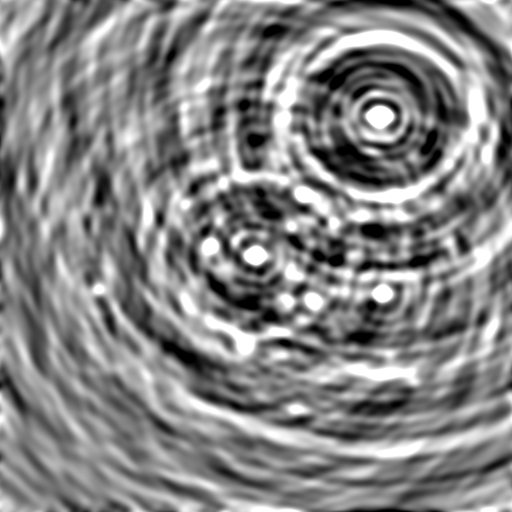
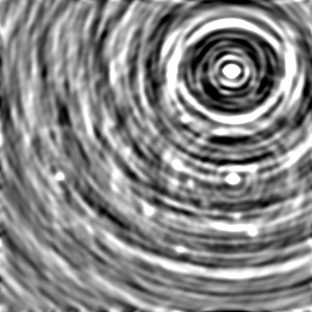
Products are below, along with the MS and sky model in case you misplaced it them. If you image corrected data you'll see what we had before, the scattering of sources with their associated sidelobes, and the dominant source towards the north west.
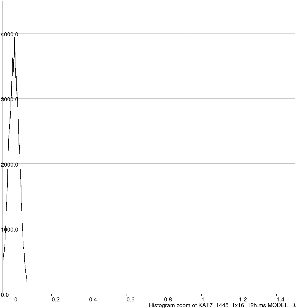
The image below is 1024 pixels covering 180 arcminutes.
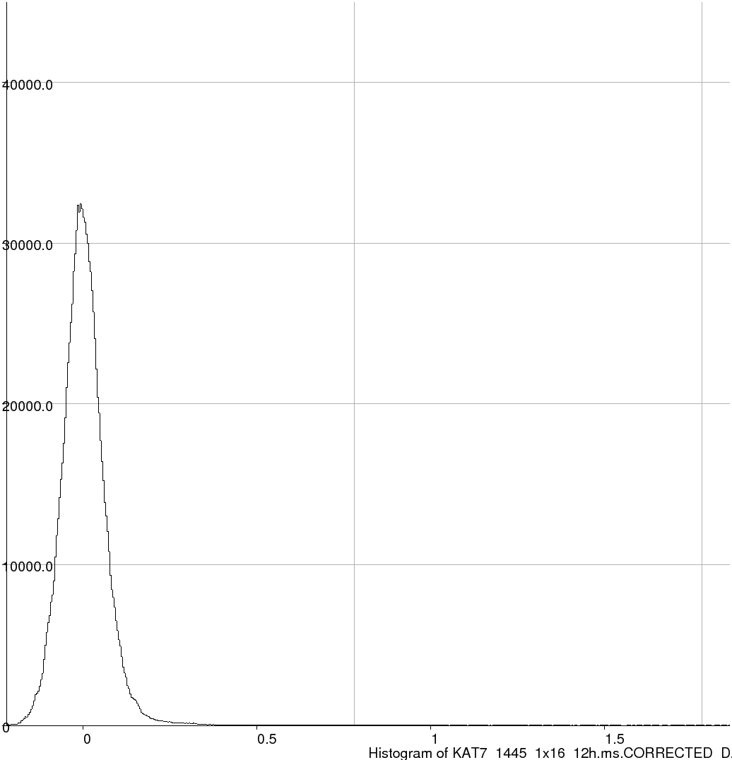
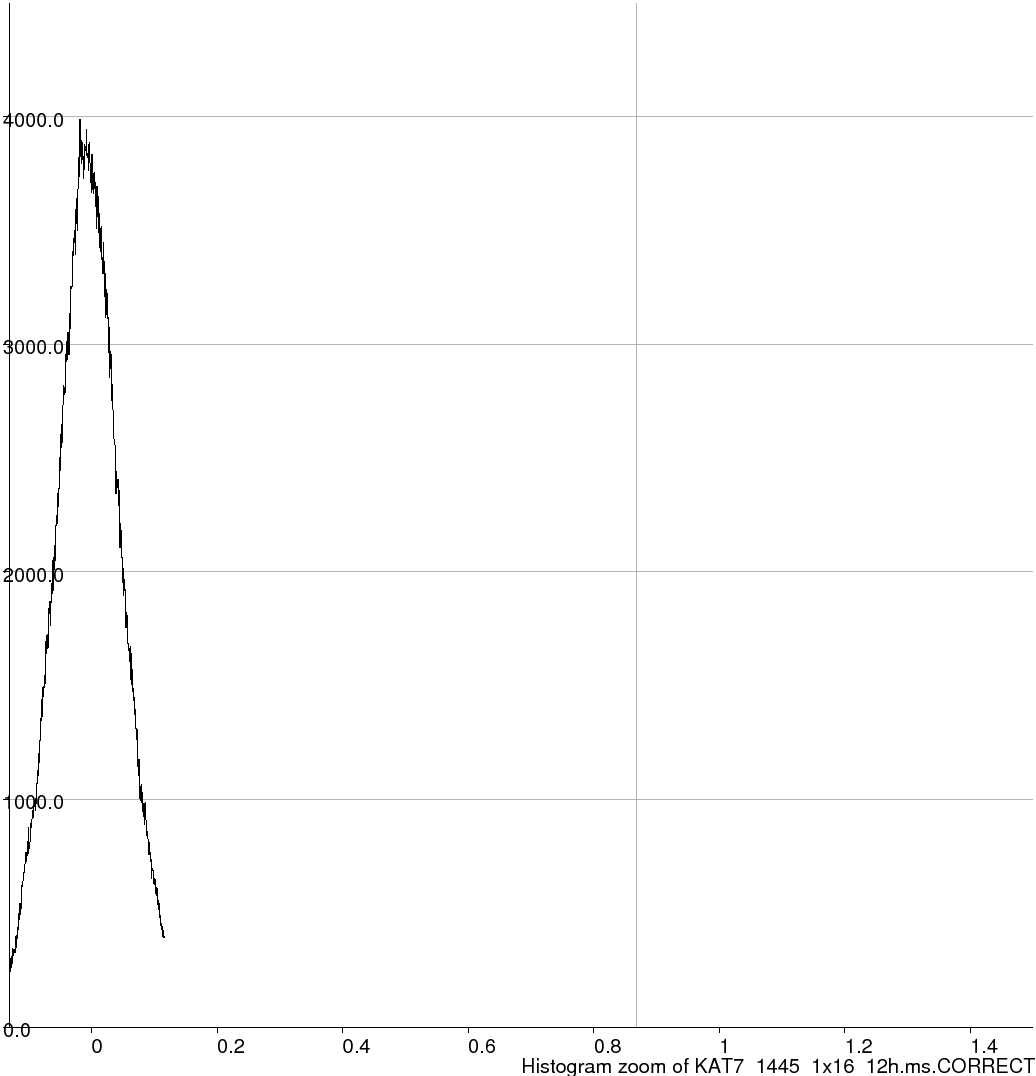
KAT7_1445_1x16_12h.ms.CORRECTED_DATA.channel.1ch.fits (header) | ||||||||||||||||
|
|
|||||||||||||||
Adding the primary beamLogged on 03/02/13 21:35:23
The turbo-sim.py TDL script that we're using here comes with a few primary beams that you can (and are encouraged) to play with. Let's repeat the simulation with the WSRT-esque cos-cubed beam model applied to this KAT-7 observation.
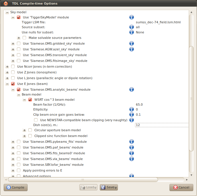
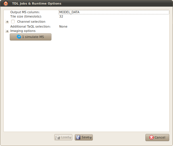
Open up the TDL Options again. Check and expand the 'Use E Jones (beam)' submenu, check and expand the "Use Siamese.OMS.analytic_beams module', expand 'Beam model' and finally check and expand 'WSRT cos^3 beam model'.
Phew. Screenshot is attached below. The only thing we've changed in this submenu from the defaults is the dish size. This just linearly scales the cos^3 beam pattern to be consistent with the 12 metre dishes that KAT-7 has.
Click 'Compile'.
One final thing: when the Runtime options window pops up, change the output column to MODEL_DATA. Open some bookmarks if you feel like it then click '1 simulate MS'.
What we have now are two simulations in the Measurement Set. The visibilities with no primary beam model live in the CORRECTED column, and the ones with the primary beam model applied live in the MODEL column.
 |
|
 |
|
Interlude: let's have a rummage in the treeLogged on 03/02/13 22:15:43
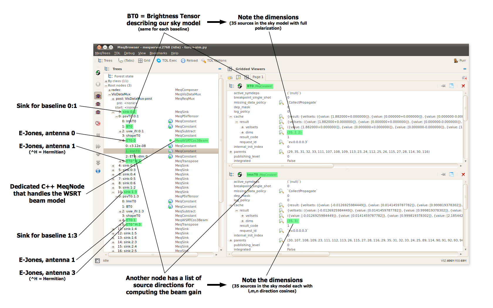
The Meqbrowser as you might expect from the name offers you the capability to browse your Measurement Equation tree.
In the 'Trees' part of the window on the left, expand the 'Root nodes', then the 'VisDataMux'.
You'll see a bunch of nodes called 'sinks'. Sinks put visibilities into your MS, and there will typically be a sink per baseline, e.g. sink:3:5 deals with the baseline formed between antennas 3 and 5.
(The nodes that read visibilities from a MS are called spigots. Since this is a regular 'sim only' simulation there aren't any of these.)
It's a good idea to try to relate what's going on in your simulation or calibration to what you see in the tree. Remember the 'onion skin' matrices in the Measurement Equation? You can hopefully see how MeqTrees implements this with the source coherency matrices at the heart of it all. The annotated diagram below might help.
 |
Screenshot-MeqBrowser - meqserver.2768 (idle) - turbo-sim.png |
 |
Make an image of your beam attenuated simulationLogged on 03/02/13 22:17:47
Once the simulation has finished it's time to make an image. Click 'TDL Exec' and expand the 'Imaging Options' submenu.
Make sure the 'Image type or column' points to MODEL_DATA and make a dirty image over an appropriate sky area. It should remember what we had from the CORRECTED_DATA run: 1024 pixels over 180 arcminutes. Make sure these are the same as that will be required for the next section.
The effects of the primary beam should be obvious from a quick look at the image. Our once proud dominant source in the north west is now pushed down into the sidelobes of the now dominant central source. The central source remains unattenuated as the beam gain here is unity.
Again, you are encouraged to play around with the deconvolution options.
|
|
|||||||||||||||
Tigger makes all the differenceLogged on 03/02/13 22:27:46
The process above (if you haven't done any cleaning experiments) should have resulted in two FITS files:
KAT7_1445_1x16_12h.ms.CORRECTED_DATA.channel.1ch.fits
and
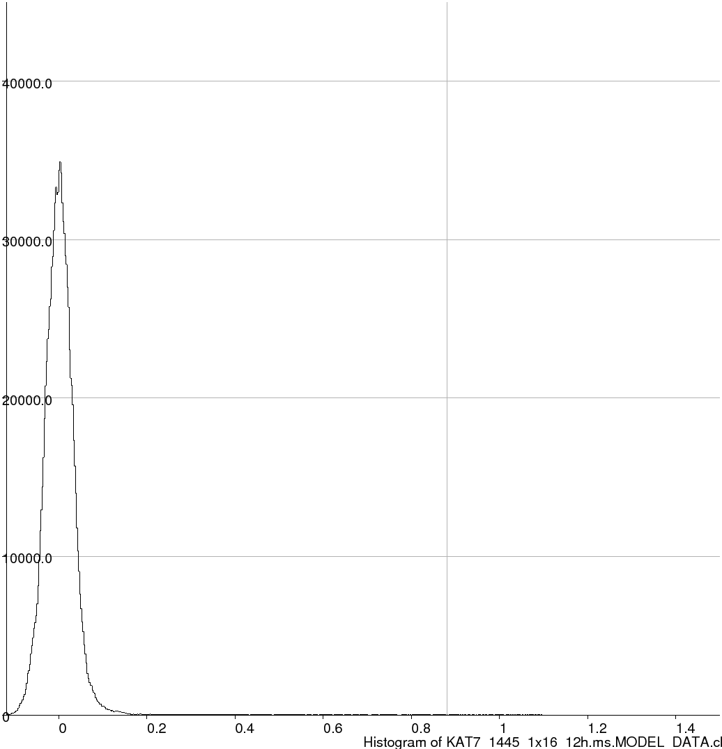
KAT7_1445_1x16_12h.ms.MODEL_DATA.channel.1ch.fits
which contain our simulation both with and without primary beam attenuation.
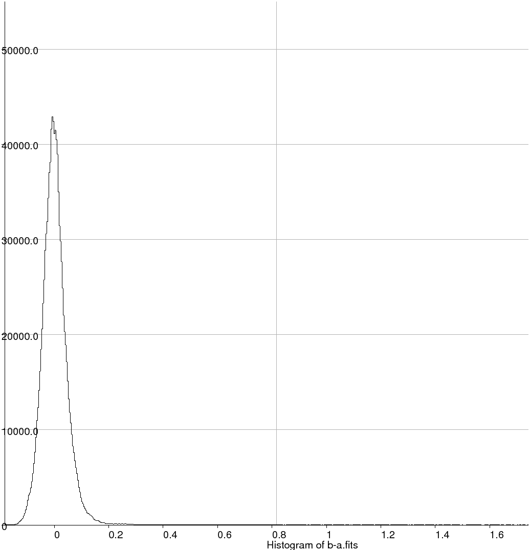
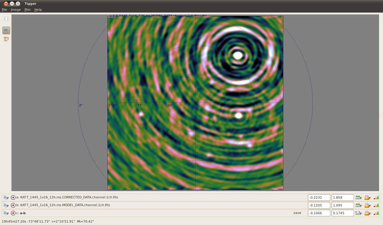
We can use Tigger to get a feel for how much intrinsic flux the primary beam has caused us to miss by making a quick difference image.
Load the first image into Tigger:
$ tigger KAT7_1445_1x16_12h.ms.CORRECTED_DATA.channel.1ch.fits
and then from the 'Image' menu select 'Load image' and locate the second FITS file. You'll see at the bottom of the screen your two images have been given 'a' and 'b' labels.
Again from the image menu, select 'Compute image'. Your images are now numpy arrays called 'a' and 'b', and you can enter any arithmetic operation into this dialogue to compute a third image 'c'.
Typing 'a-b' and hitting enter will provide a difference image. The brightness of the sources in this third image is the flux that is missing due to primary beam attenuation. You can open the sky model from the 'File' menu if you want help finding the sources.
You can also save this image as a FITS file by finding the appropriate option in its submenu in the main 'Image' menu.
 |
||||||||||||||||
|
|
|||||||||||||||
 This log was generated
by PURR version 1.1.
This log was generated
by PURR version 1.1.