The trouble with variable sources

We previously simulated a simple version of the primary beam as one of the fundamental direction dependent effects in an interferometer observation. As mentioned in the intro to that simulation, the beamshapes themselves are often complicated, with structure extending beyond the main lobe. They are naturally functions of frequency (although that can also involve subtle effects that are not obvious) but they can also be strongly time dependent. How they vary in time can also vary as a function of direction, so traditional '2GC' calibration where a single complex gain correction is applied to each antenna (or each feed) won't correct the sources that are blighted by this.

(Primary beams also introduce instrumental polarization effects: the elements in the array generally have a pair of dipoles that are sensitive to orthogonal modes of polarization. For aperture arrays the projection effects can lead to the instrumental polarization being quite severe, and for dish arrays it is definitely not neglible as the two receptors can never be co-spatial in the optical focal point.)

Although the title doesn't suggest it, this section introduces something that is very important in the context of direction dependent effects. Your interferometer doesn't care if a source is actually flaring over the course of your observation due to some astrophysical process, or if it's apparently variable due to an instrumental effect. Either way, they will both cause problems in your continuum image.

Here we simulate a source that flares over the duration of the observation. It's probably unlikely that a real radio source would do what we're about to pretend it does, and an instrumental effect is also unlikely to cause this, but it illustrates the point nicely. It also introduces the power of additive (or subtractive) simulations.

Again we're starting from a familiar place, namely the end point of the 'beam me up' simulation. I kind of wanted these simulations to be individually self-contained, but that's just not practical.

The ingredients for this one are our MS (attached), our sky model (also attached) and the WSRT cos^3 beam model applied at compile time with the 12 m dish correction.

One slight difference to make sure you're awake: in the 'Output MS column' enter 'DATA' into the 'custom' field.

The turbo-sim.py script has a simple module for adding transient sources with Gaussian light curves. What we're going to do here is take the existing visibilities that we just wrote to the DATA column and add the visibilities corresponding to a flaring source at the phase centre to them. This will effectively make our existing central source flare.

We'll do this in two stages though to make it more interesting.

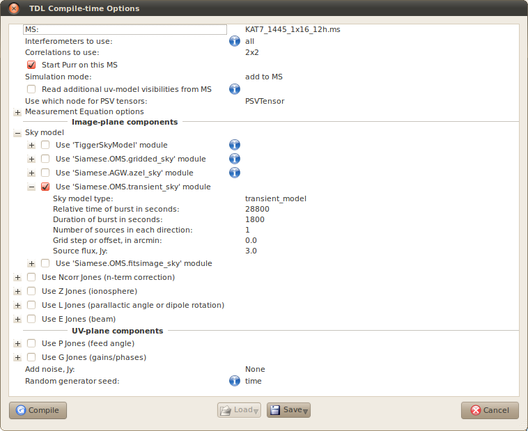
Hit the 'TDL Options' button to bring up the compile time menu. The vital thing to do here is change the 'Simulation mode' option to 'add to MS'.

In the 'Sky model' menu, disable the 'Use TiggerSkyModel module' option and check the 'Use Siamese.OMS.transient_sky module' option. Here you can specify a few simple options to simulate a flaring point source.

Select 'transient_model' for 'Sky model type'. As mentioned previously, the light curve follows a Gaussian. You can specify the peak time of the burst from the start of the observation (in seconds) and the half maximum duration of the burst (in seconds). You can also specify the source flux. The offset option is getting set to 0.0 because I'm faking this for the central source.

I set the options up as per the screenshot below, but as always you are encouraged to play around.

Finally, disable the 'Use E Jones (beam)' option. This will make absolutely no difference other than making the simulation leaner, although on a problem of this size you would probably not notice the difference.

Press 'Compile'.

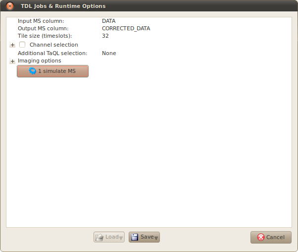
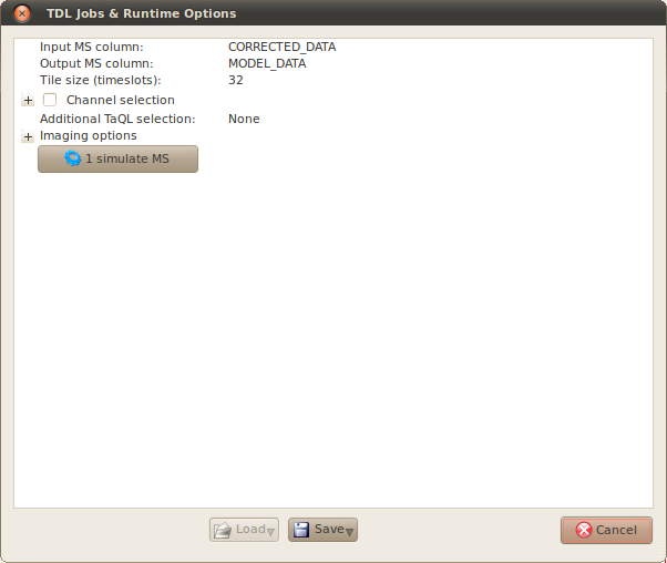
Now another slight difference from what we've done before. You'll see (as per the screenshot below) that the run time options now have an 'Input MS column' thanks to us specifying 'add to MS' at compile time.

What we want to do here is take the DATA column visibilities, compute the visibilities from the simulation, add the results together and write these values to the CORRECTED_DATA column.

Click '1 simulate MS' and this should happen.

There's only one thing more interesting than a Gaussian, and that's TWO Gaussians. Here we're essentially repeating the process, except we're taking the now-flaring visibilities in CORRECTED_DATA, adding another burst of activity to the central source slightly later on in the observation and writing the result to MODEL_DATA.

Again the 'add to MS' option needs to be selected in the compile time menu, and the parameters for the transient source need tweaking, e.g. as per the screen shot below. Here I've added a second burst later in the observation.

Again there's a slight modification to the runtime options: the input MS column is now CORRECTED_DATA and the output MS column is now MODEL_DATA.

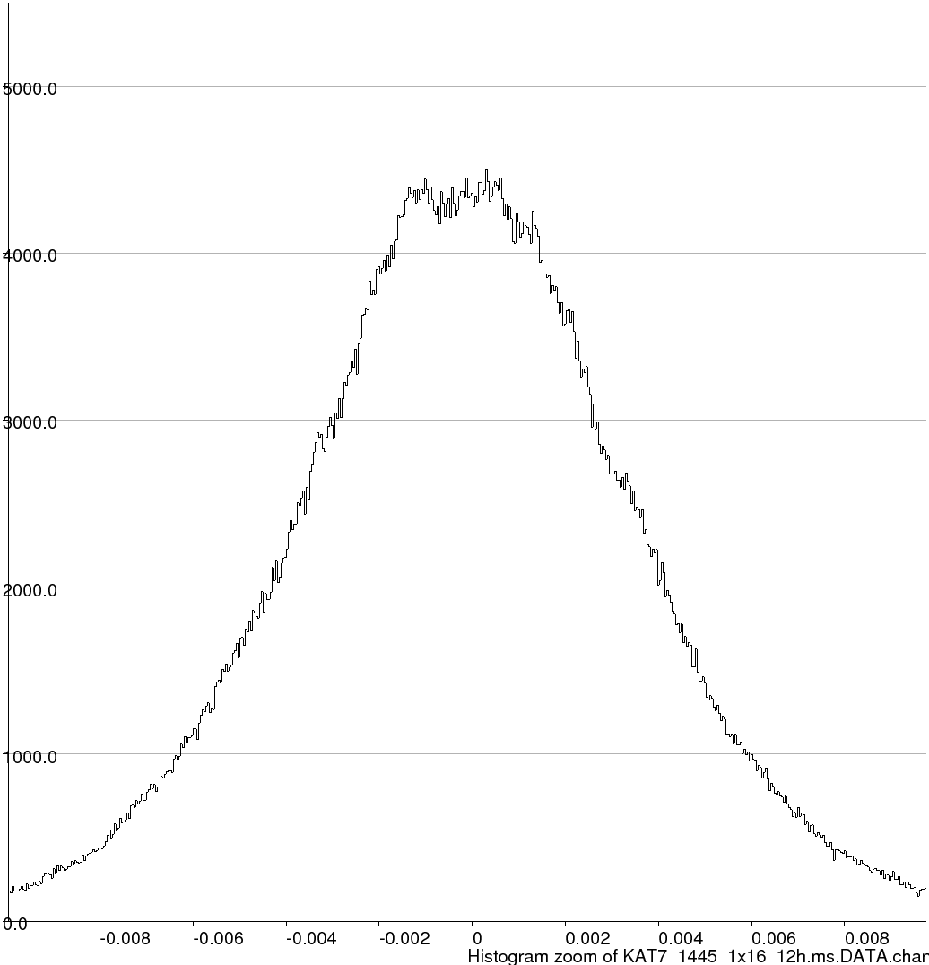
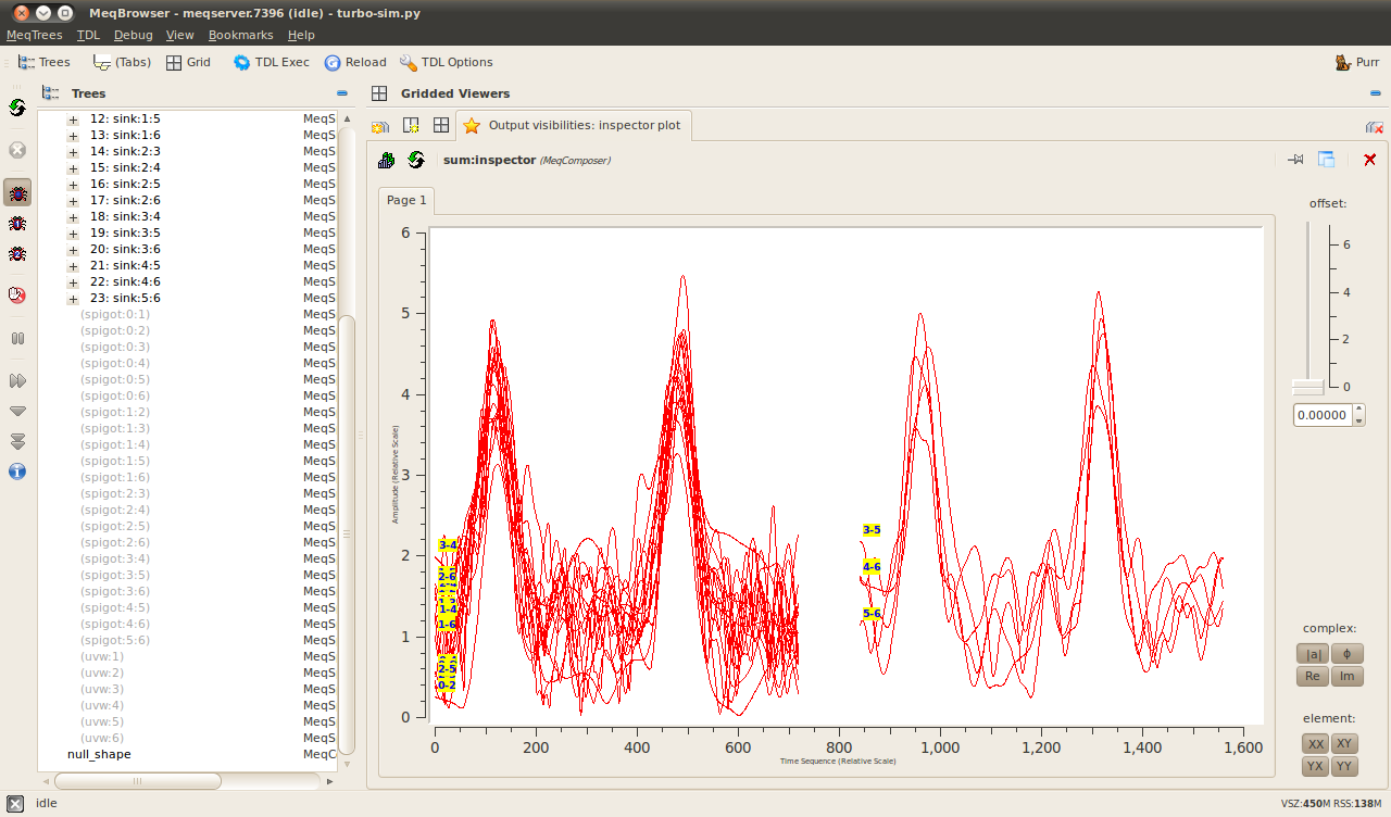
Before you hit '1 simulate MS' however, open the 'output visibilities: inspector plot' bookmark from the menu. I've screen shotted the Meqbrowser window below with the output amplitudes being plotted per baseline. It's hopefully rather obvious what the effect of adding these two bursts to them is.

(Aside: on the left in the browser you can see there are some spigots as well as sinks in the tree. This is an additive simulation remember, so MeqTrees has to read some visibilities from the Measurement Set to compute what it's going to write back to it afterwards.)

We've now got a Measurement Set that contains the unperturbed sky in the DATA column, a single flare in the CORRECTED column and the double flare scenario in the MODEL column.

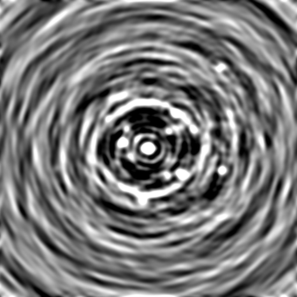
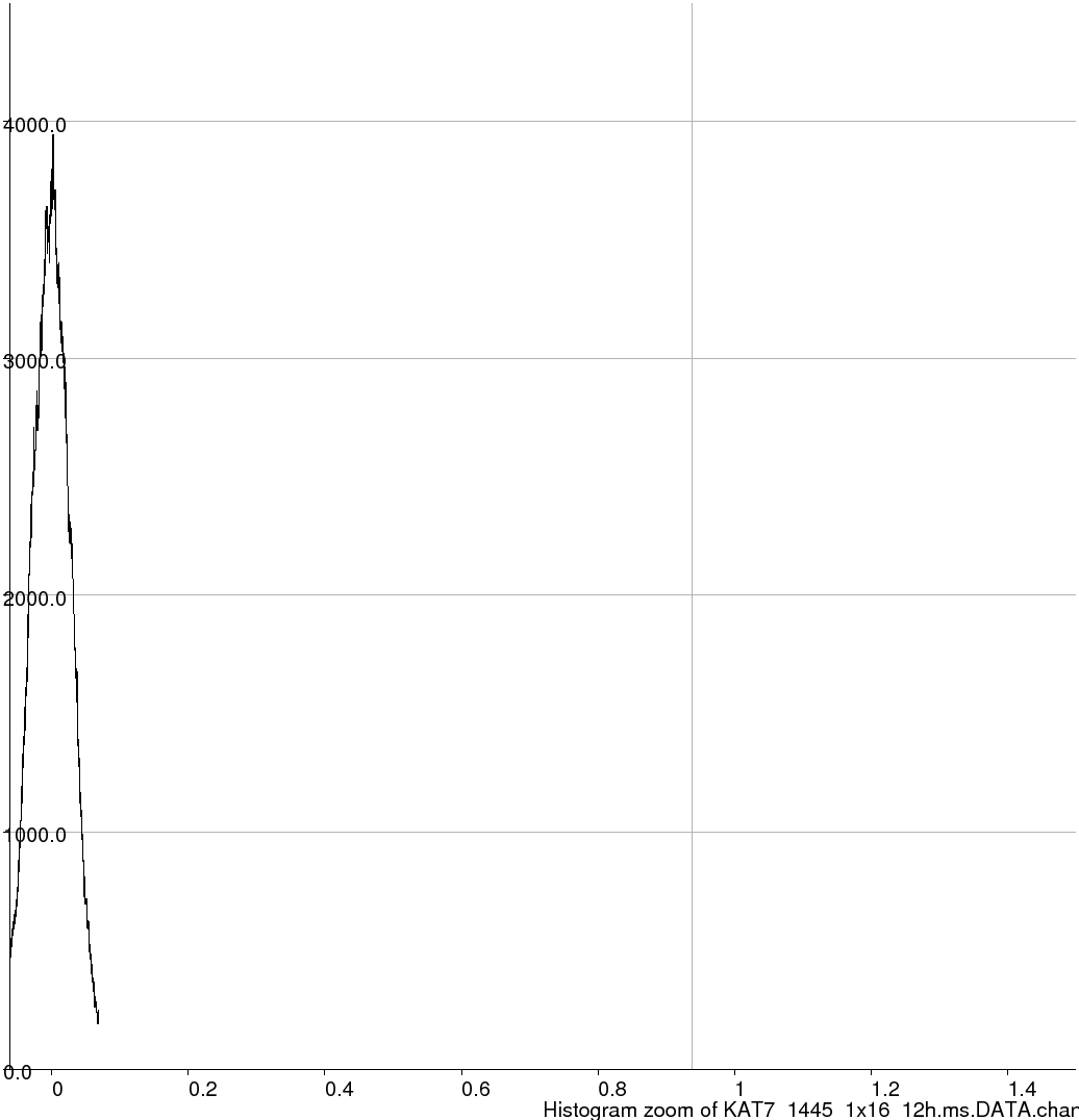
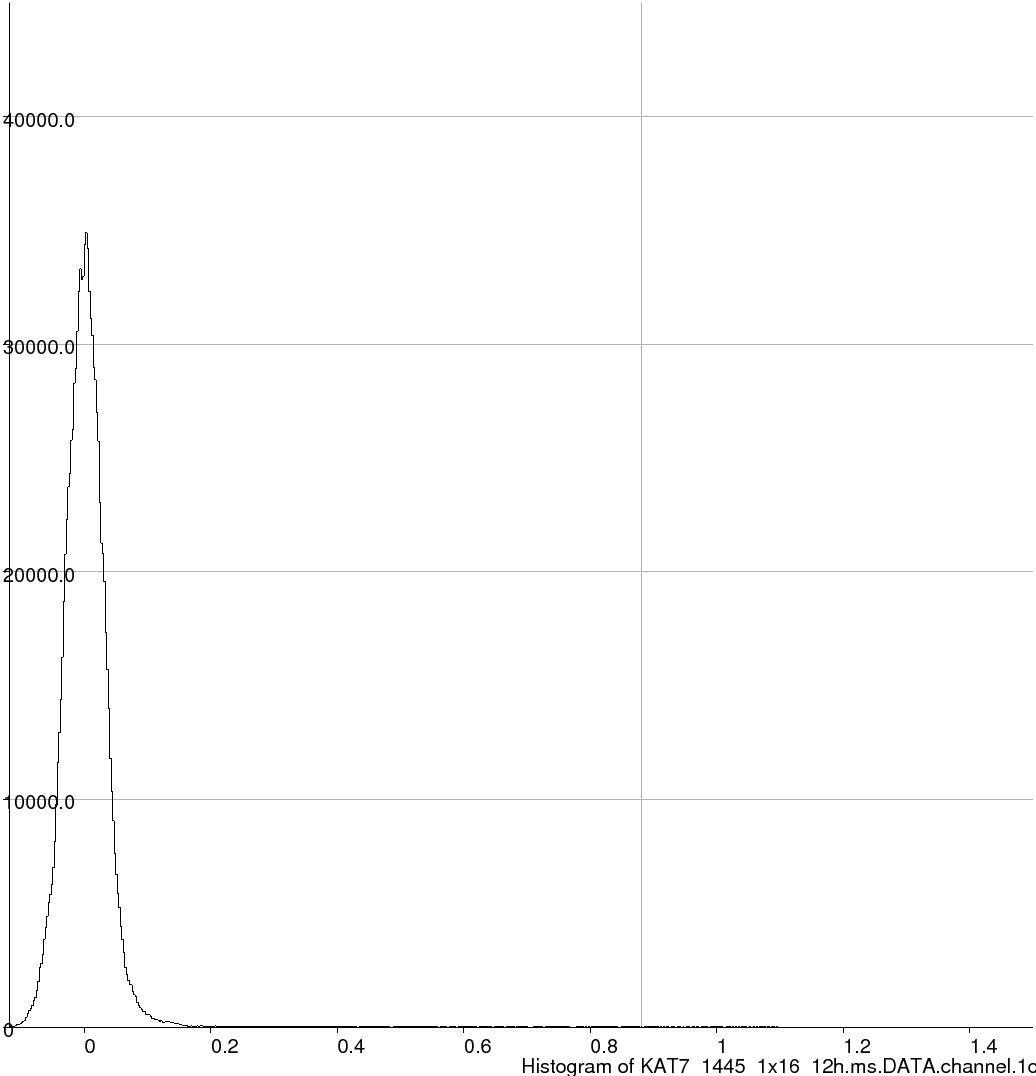
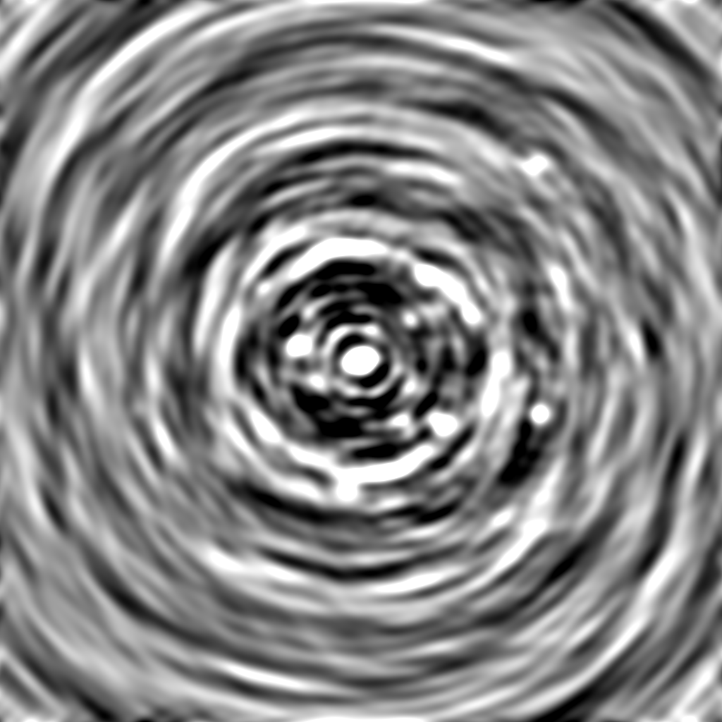
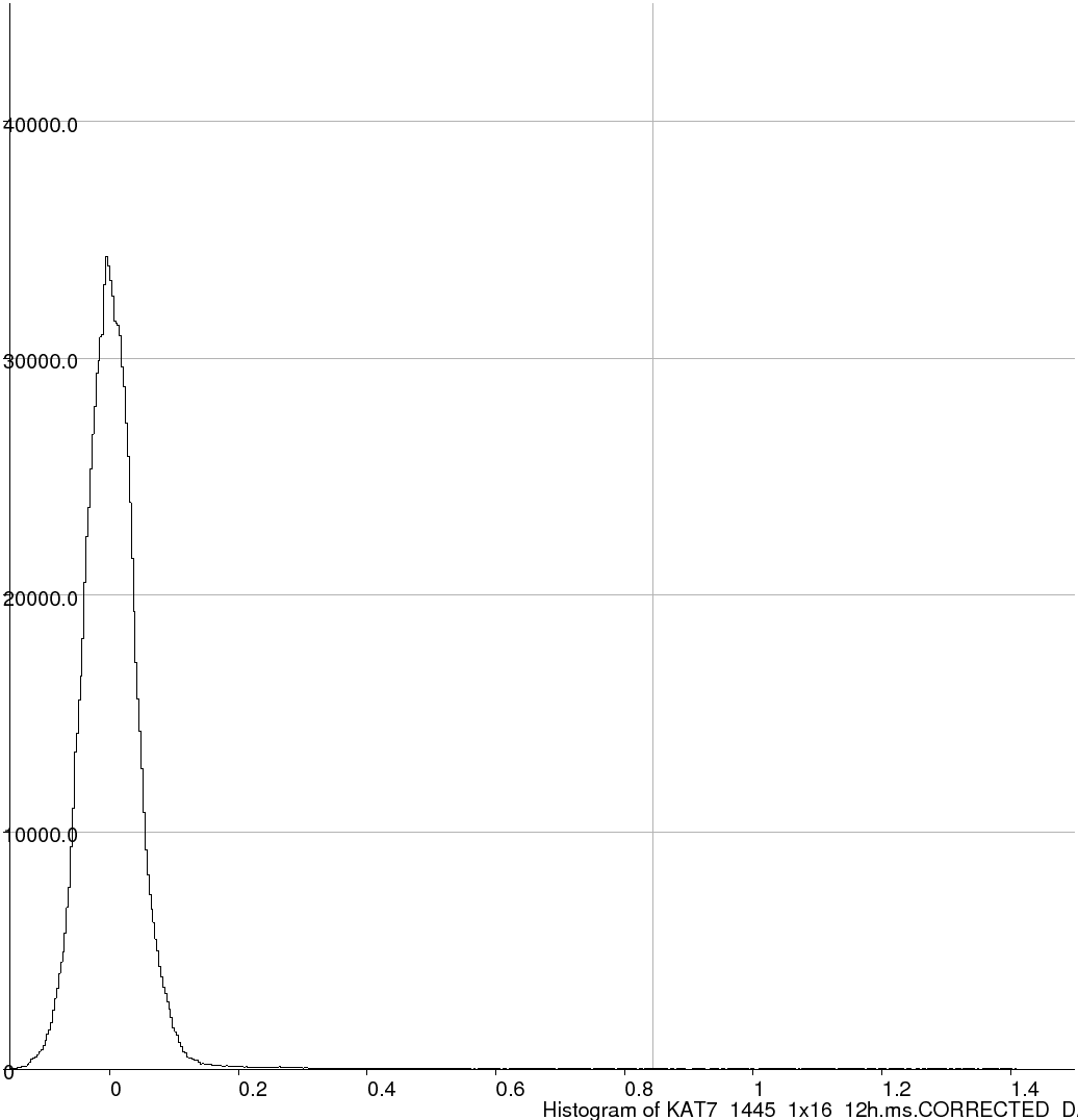
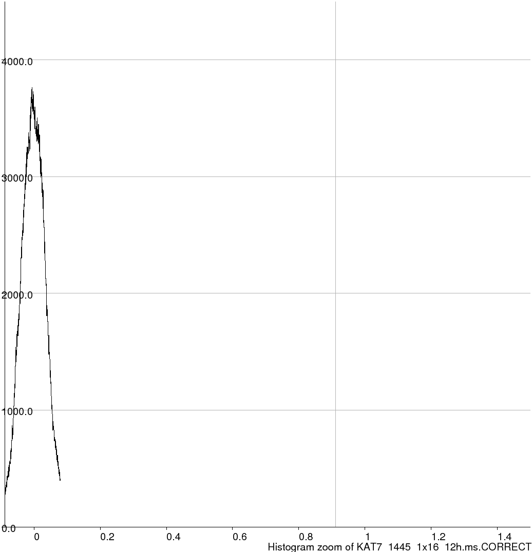
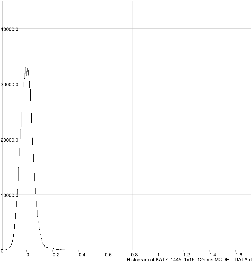
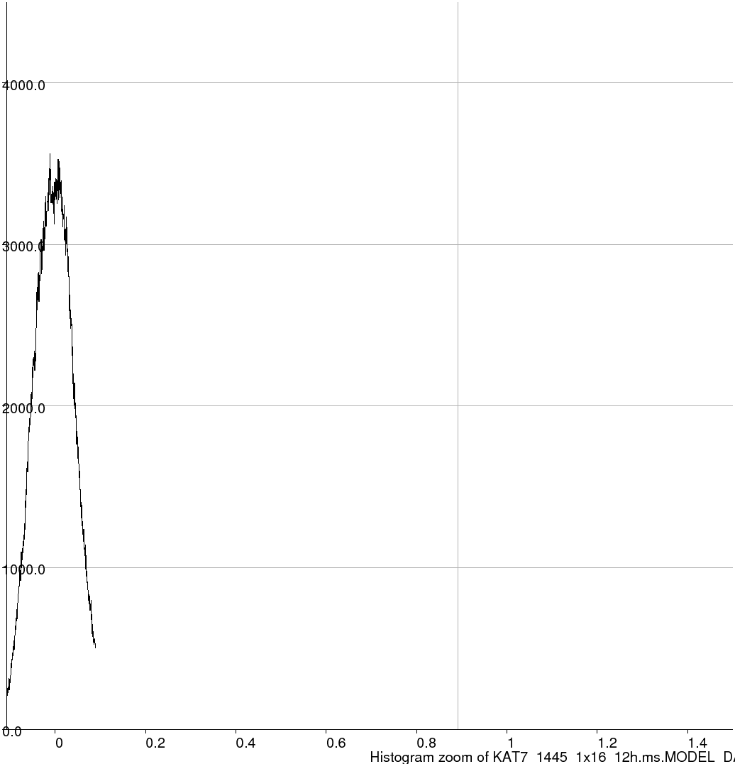
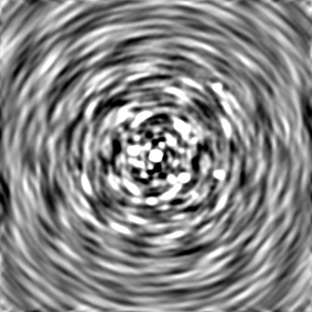
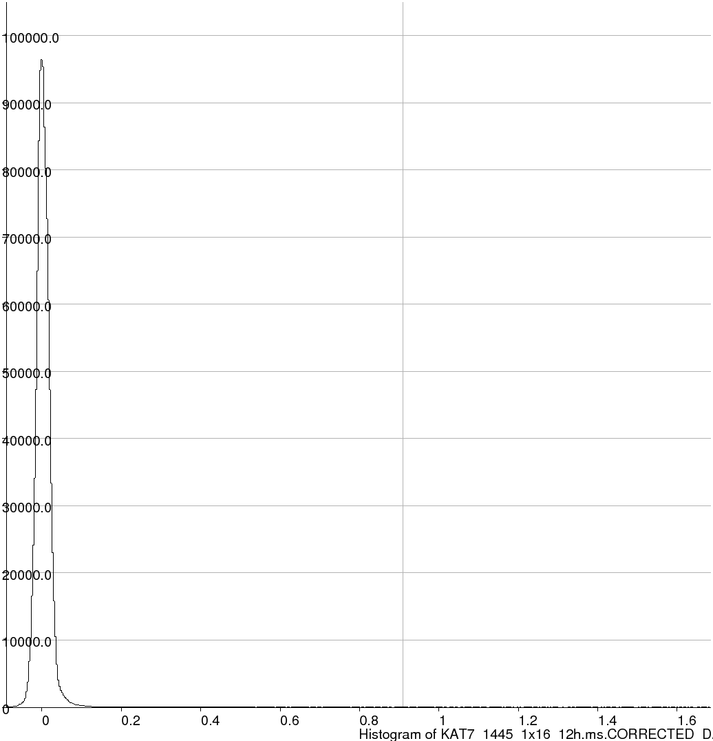
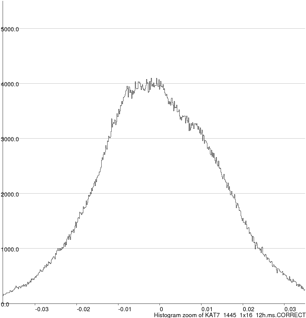
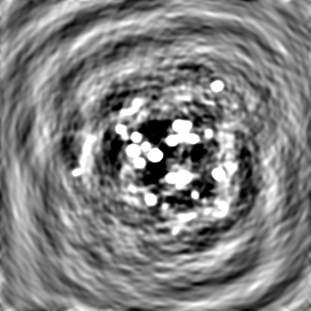
Making an image of all three of these should allow us to see the situation deteriorate. A quick look at the sigma values on the Purr rendering of the FITS images below shows how the situation gets progressively worse. The biggest cause in the increase of these values is the PSF sidelobes associated with the bright source. The sidelobes exist at some fraction of the brightness of the main lobe for the PSF. Times during which source has flared end up with correspondingly higher sidelobes in PSF for those time slots. The PSF associated with this source now differs from the assumed 'analytic' PSF that one obtains by Fourier transforming the Fourier plane sampling pattern.

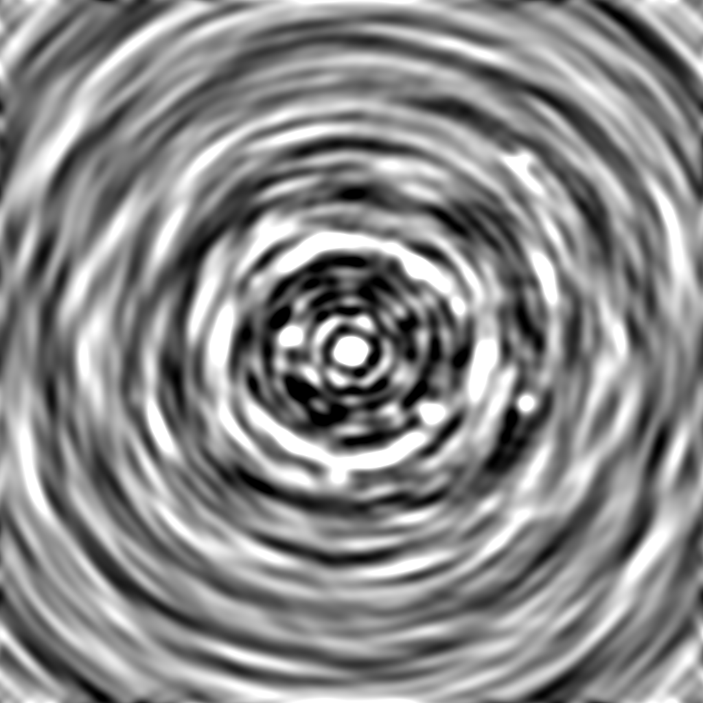
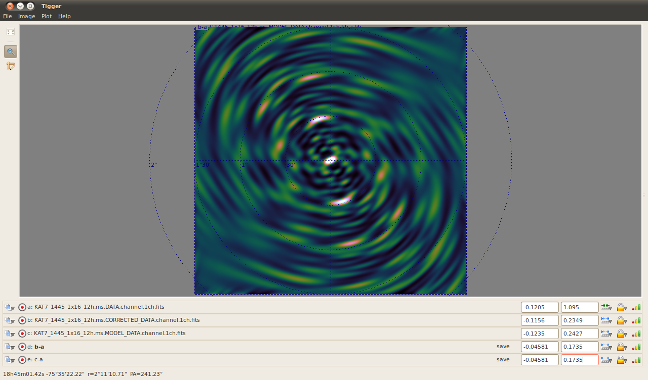
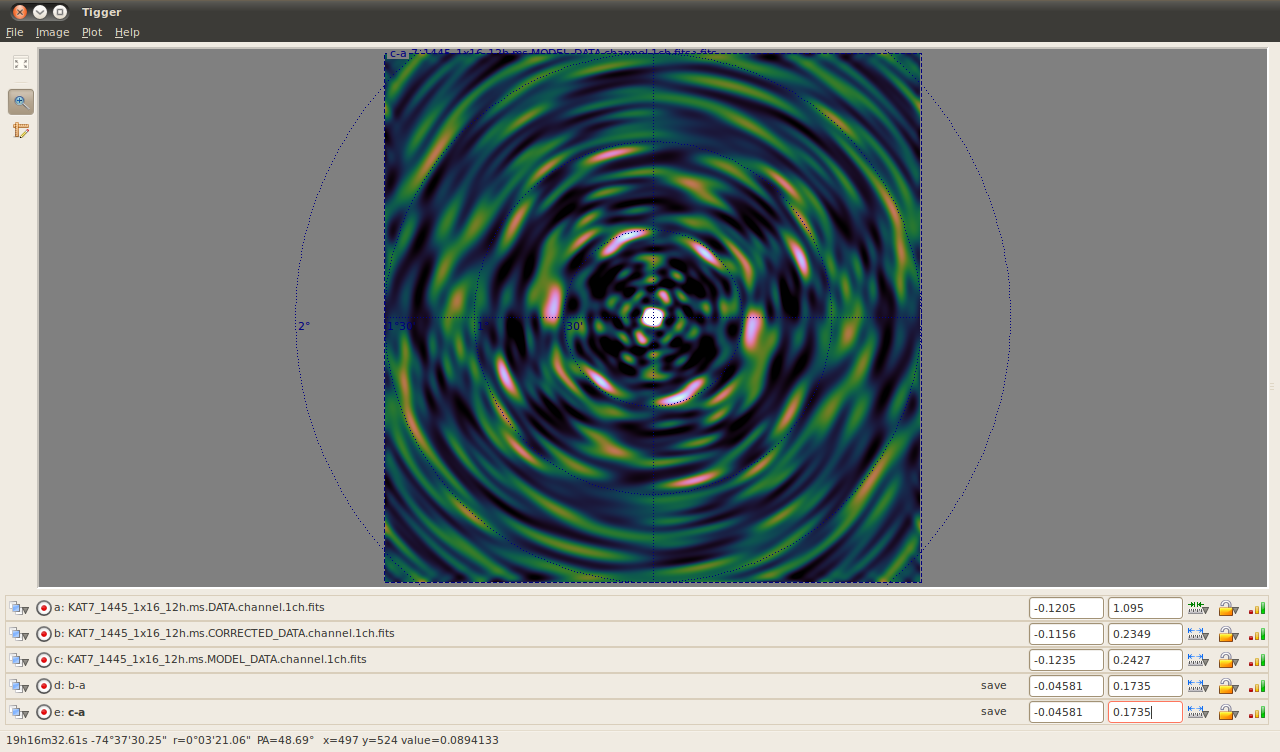
Again I've made some difference images in Tigger using the images formed from each column in the MS. This makes it easier to see. The screenshots below show CORRECTED minus DATA and MODEL minus DATA, showing how each individual flare adds extra bright regions to the sidelobes of this source.

Yeah, good luck with that.

The CLEAN algorithm relies on the PSF being identical to the analytic PSF for every point in the image. For the central source with its partially inflated sidelobes it won't be successful, and will leave residual PSF-like emission around it.

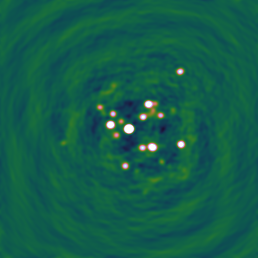
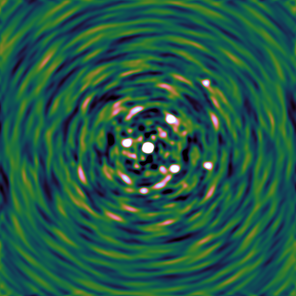
You can see the result below for both the unperturbed sky and the double flare sky. Note again the sigma values in the Purr FITS renders. Awesome as Purr is it often doesn't do the most photogenic job of making PNG out of a FITS file, so I've attached two images (on the same colour scale!) below, exported directly from Tigger.

This residual PSF emission around sources is usually a good sign that something is amiss (unless of course you are interested in astrophysical transients -- you don't want to calibrate out your Nature paper).

Can you think of a calibration approach that would take care of this problem?

Note that the CASA imager / lwimager will only perform a clean operation on the CORRECTED column of a Measurement Set, so I had to play a quick game of "Musical Columns" to get the images below.