Source colourization through the primary beam

We mentioned during the 'Beam me up' simulation that the primary beam pattern scales with frequency, and it is this property that we are going to investigate with this simulation.

We will start once again with the KAT-7 array, however we're going to take out the 12 metre dishes, and give it 25 metre VLA dishes instead. Also, instead of a simplistic analytic formula for the primary beam, we're going to use simulated beam patterns read in as FITS files. MeqTrees has the capability of reading in such files and performing interpolation, as well as adding rotation effects that simulate the rotation of the beam pattern on the sky due to the azimuth-elevation mounts of the VLA antennas.

The beam patterns themselves are a bit closer to reality than what can be achieved with a simple analytic approximation for the VLA beam. (Note that the cos-cubed function used previously does a very good job of representing the main lobe of the WSRT beam, however the WSRT is famed for its stable beam, thanks in part to its equatorial mount system.) The beam FITS images we'll use here are generated by Walter Brisken's Cassbeam software which uses ray tracing to compute the beam patterns of Cassegrain dishes. It performs the calculation in full polarization, and the end result is a complex-valued 2x2 Jones matrix describing the response pattern of the dish to incoming radiation.

A visualisation of such a beam pattern (in this case at 1.265 GHz) is attached below (the colour scale maxes out with purple). A complex valued (in this case amplitude and phase) 2x2 matrix thus results in eight FITS images to full describe the beam. As you can see there is some complex structure away from the main lobe that is not azimuthally symmetric. This arises as radiation scatters off the support struts that hold the secondary reflector for the Cassegrain optics. The VLA antennas have four of these support legs giving rise to the 4-fold symmetry of the first sidelobe.

We're also going to give our observation a bandwidth of 1 - 2 GHz (also the same as the VLA L-band bandwidth). This gives a fractional bandwidth, defined here as the ratio of the bandwidth to the centre frequency, of about 67%. The higher this percentage is, the more significant you can expect the frequency-related effects across the band to be.

For this simulation we select six frequencies across the band: 1.0, 1.2, 1.4, 1.6, 1.8 and 2.0 GHz. Attached below are six KAT-7 Measurement Sets at these frequencies, each with a single 50 MHz channel, and again using a 12 hour track.

To see the effects of the beam we also need six beam patterns at the relevant frequencies. We'll take a bit of an ideal-world shortcut here to make the problem leaner, and discard the beam patterns that include the cross-hands of polarization (XY and YX). This is how you would ideally like your instrument to behave: your instrumental Jones matrices all having unity gain on the XX,YY (or LL,RR; or HH,VV) diagonals (or at least the sort of decent behaviour that can be replicated with a little bit of linear algebra), and zeros on the XY,YX (or LR, RL; or HV; VH) off diagonals, that is to say the instrument does not interfere with your polarization measurements at all. In reality the E-Jones matrix of your antenna will stamp its authority on your the polarization state of the incoming radiation.

The pair of feeds that are sensitive to the two orthogonal polarization states are separate entities and thus can't be co-spatial, and this always results in some sort of instrumental polarization, manifested by the patterns in the XY and YX plots below. The more eagle-eyed reader might be able to discern a slight offset between the amplitude peaks of the XX and YY images in the image below. Find a VLA person and ask him or her about beam squint.

(The same VLA person will probably also point out that we're using linear X/Y feeds when in reality the VLA has circular L/R feeds, but don't worry, it's a simulation and we're omnipotent. You can always point out that the VLA doesn't consist of seven antennas in the Karoo either so the feed setup should be the least of their complaints.)

Anyway, our raw materials are 6 Measurement Sets at the relevant frequencies, and 6 x 2 x 2 FITS images describing the real and imaginary parts of the beam patterns (2) for the diagonal terms of the Jones matrix (2) for each of the (6) frequencies.

We'll also need a sky model, and for this simulation I've cooked up a LSM (beam_freq.lsm.html) that has six sources in it that steadily increase in radial distance from the phase centre in a pattern that vaguely resembles a spiral.

All of these products are attached below.

The point of this simulation is to get a feel for the effects that the primary beam has not only on the brightness of sources in the field (as per the 'beam me up' simulation) but also how it affects their frequency behaviour.

We want to therefore simulate the intrinsic properties of the source, then simulate the apparent properties and contrast the two.

As always, there are numerous ways to approach a problem. I'm not saying the following method is the best one but it does the trick.

1) We're going to simulate the instrinsic and apparent properties for the lowest frequency by hand, that is by doing what we've been doing so far and clicking buttons in the Meqbrowser.

2) To do the same thing for all frequencies, i.e. opening each of the Measurement Sets, finding the beam patterns, clicking the 'make image' button etc. isn't exactly a big job, but that's because we've only got six channels and seven antennas. So we're going to take the by-hand operation and script it using the excellent batch mode operation that MeqTrees offers.

3) Once that's done, we want to plot the spectrum of each source by measuring the brightnesses in the maps. Again this could be done by hand, but scripting it makes life a lot sweeter.

If you "tar -xzvf" the beam pattern and Measurement Set archives that are attached to this Purr log you should end up with the following Measurement Sets in your (hopefully freshly created and dedicated to this simulation) current location:

KAT7_1000_1x50_12h.ms

KAT7_1200_1x50_12h.ms

KAT7_1400_1x50_12h.ms

KAT7_1600_1x50_12h.ms

KAT7_1800_1x50_12h.ms

KAT7_2000_1x50_12h.ms

The first number after the KAT7 is the frequency of the MS in MHz (the following items in the names tell you that there is 1 x 50 MHz channel and that the observation is 12 hours). There should also be a beam_patterns folder that contains the following files:

fitsbeam_L1000_xx_imag.fits

fitsbeam_L1000_xx_real.fits

fitsbeam_L1000_yy_imag.fits

fitsbeam_L1000_yy_real.fits

fitsbeam_L1200_xx_imag.fits

fitsbeam_L1200_xx_real.fits

fitsbeam_L1200_yy_imag.fits

fitsbeam_L1200_yy_real.fits

fitsbeam_L1400_xx_imag.fits

fitsbeam_L1400_xx_real.fits

fitsbeam_L1400_yy_imag.fits

fitsbeam_L1400_yy_real.fits

fitsbeam_L1600_xx_imag.fits

fitsbeam_L1600_xx_real.fits

fitsbeam_L1600_yy_imag.fits

fitsbeam_L1600_yy_real.fits

fitsbeam_L1800_xx_imag.fits

fitsbeam_L1800_xx_real.fits

fitsbeam_L1800_yy_imag.fits

fitsbeam_L1800_yy_real.fits

fitsbeam_L2000_xx_imag.fits

fitsbeam_L2000_xx_real.fits

fitsbeam_L2000_yy_imag.fits

fitsbeam_L2000_yy_real.fits

plus a small and possibly pointless readme file. The first number in the filename is again the frequency in MHz and the rest of the name tells you which polarization the beam pattern is relevant for and whether they are real or imaginary components. Remember we have ditched the cross polarization products for this simulation. These are regular FITS files so you can explore them using Tigger, although remember the difference between real and imaginary and amplitude and phase; they won't look like the patterns plotted in the first section of this log.

The first thing we're going to do is simulate the intrinsic sky so you can see the layout of the sources. Hopefully opening the meqbrowser, connecting to a server and loading up turbo-sim.py should be a familiar process by now!

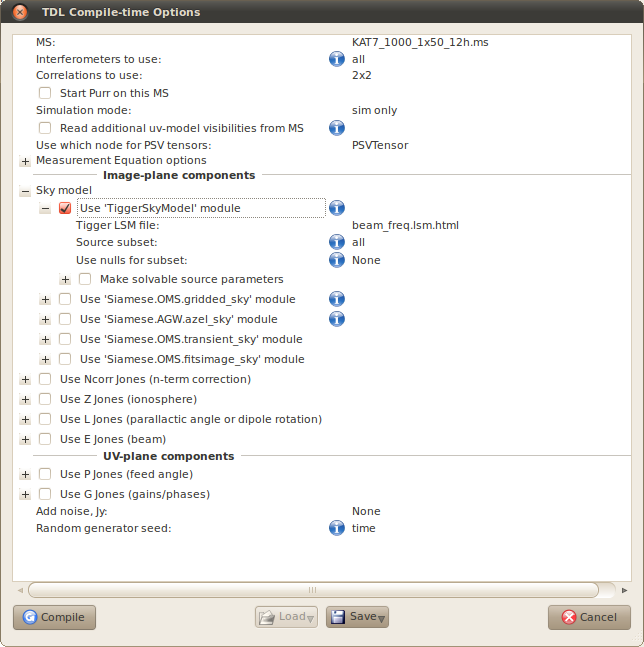
Once you're there, we need to select a Measurement Set. Let's start at the lower edge. Point the MS field to KAT7_1000_1x50_12h.ms, expand the 'Sky Model' section, check "Use 'TiggerSkyModel' module" and point the 'Tigger LSM file' field to beam_freq.lsm.html. Everything else is left unchecked.

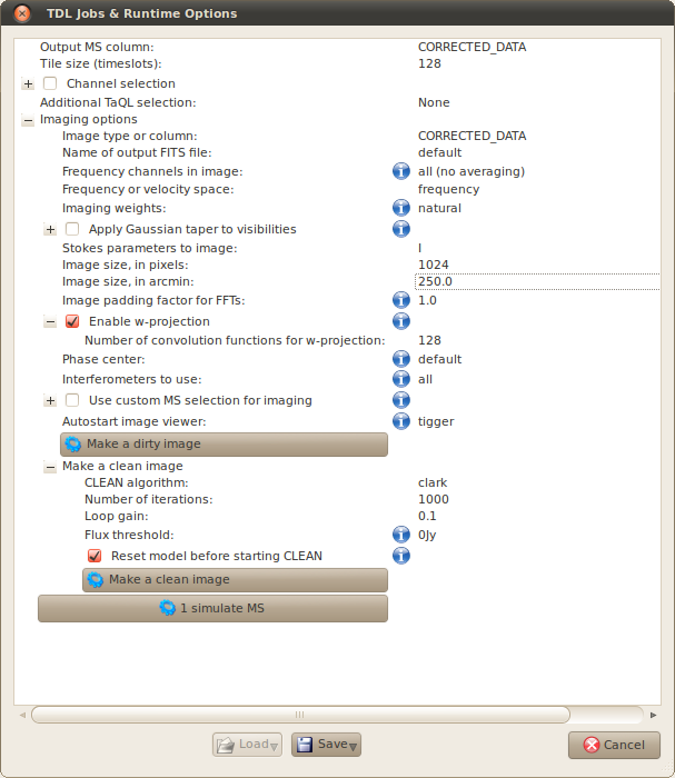
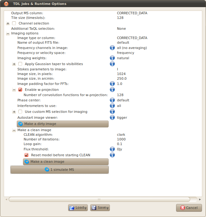
Click 'Compile'. Open a bookmark if you feel like it (always useful when a simulation is this fast just to check that it's actually calculated something), and click '1 simulate MS' to write the data to the CORRECTED_DATA column.

Once this has finished, click 'TDL Exec' again and make a clean image with a few hundred components. When we compare the intrinsic vs apparent spectra in the sections that follow we'll want to use deconvolved images.

Have a think about why a dirty image won't be suitable, before this gets explained later on in this PURR log. In the mean time you might want to rename the restored image to something other than the default. We have to make cleaned images, which means we have to use the CORRECTED data column, which means that when we image the simulation in the next section this will get written over. (We'll address this issue when we automate the other frequency channels shortly.)

Finally, and this bit is important, bring up the 'TDL Exec' window and click the save button at the lower edge. Click 'new profile' and give it the name 'source_colourization_intrinsic'. This will write your simulation and imaging parameters to tdlconf.profiles under the heading you have specified.

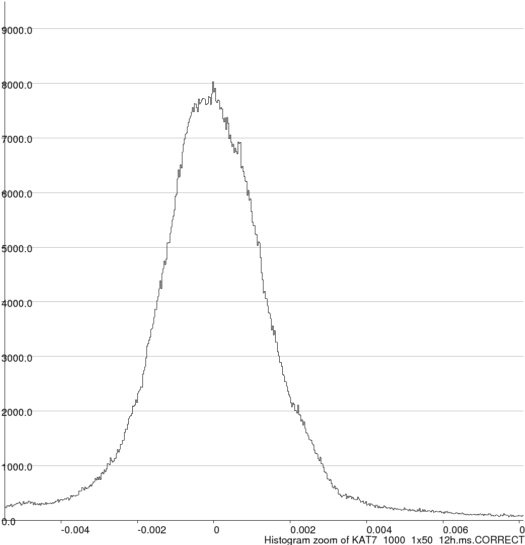
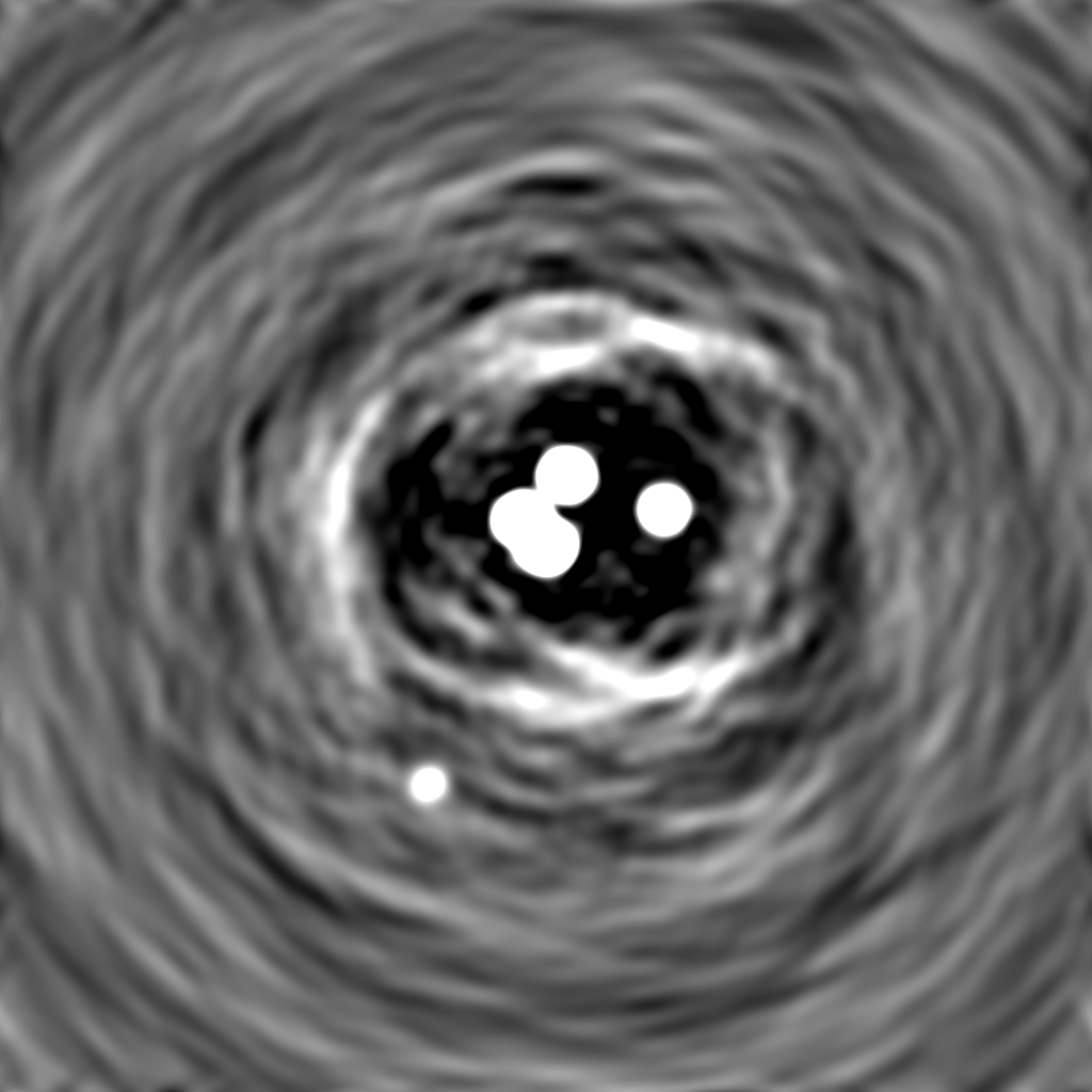
A standalone .tdl.conf file for this simulation is attached below. You should also be able to see the loose spiral pattern that I gave the sources in the FITS file rendering.

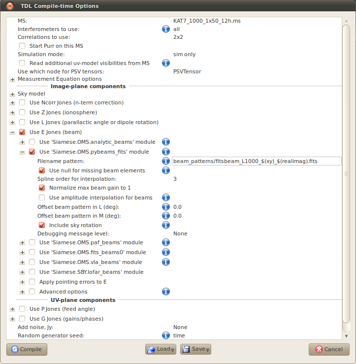
Now let's apply our simulated beam patterns to the simulation. Bring up the compile time options again and expand the 'Use E Jones (beam)' submenu. Check the "Use 'Siamese.OMS.pybeams_fits' module" option. Hovering the mouse pointer over the little 'i' information icons in the browser is always useful, and in the case of the 'Filename pattern' of this module, particularly so.

The beam patterns are specified here, and MeqTrees will substitute certain parts of the filename string that you enter, allowing you to specify mutliple correlation product beams, and also real and imaginary components in only one parameter.

In our example we are using:

beam_patterns/fitsbeam_L1000_$(xy)_$(realimag).fits

assuming the beam patterns are still in the beam_patterns folder. We're using the patterns appropriate for the 1000 MHz simulation (i.e. this MS). Instead of $(xy) when the simulation compiles, MeqTrees will loop over 'xx', 'xy', 'yx' and 'yy' into the filename, and similarly instead of $(realimag) it will loop over 'real' and 'imag', thus utilising the appropriate beam pattern at the appropriate place.

A couple of other options here are also pretty important. We want to check 'Use null for missing beam elements', as you will recall we are not using cross polarization beams, so MeqTrees will just assume these have zero gains. I've also checked 'Normalize max beam gain to 1', which fixes the boresight beam gain to unity.

Finally, another important option: ensure that you have checked 'Include sky rotation'. This rotates the beam pattern on the sky as the observation progresses as is the case for a genuine observation with an alt-az mount.

Click 'Compile', open a bookmark if you want, ensure we are writing to CORRECTED_DATA and then click '1 simulate MS' to write the visibilities.

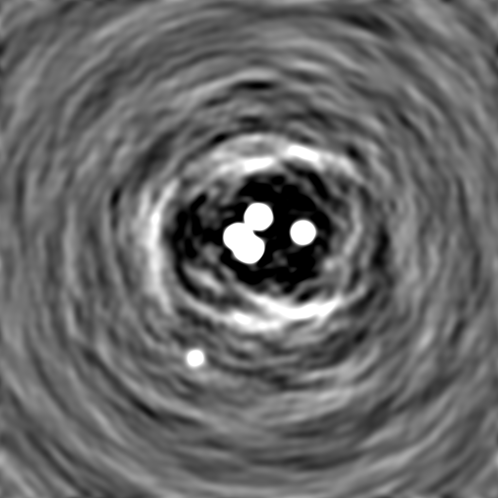
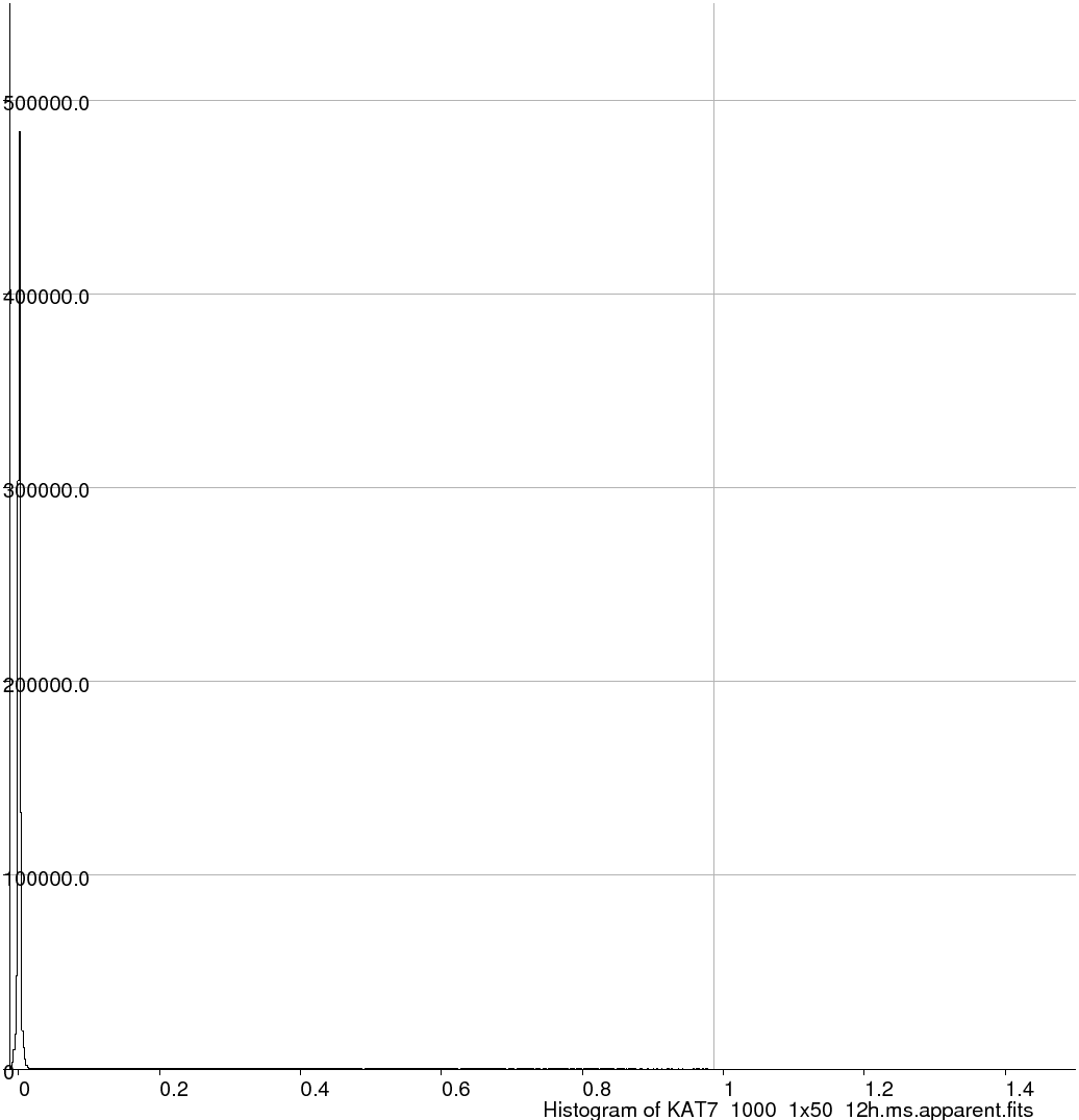
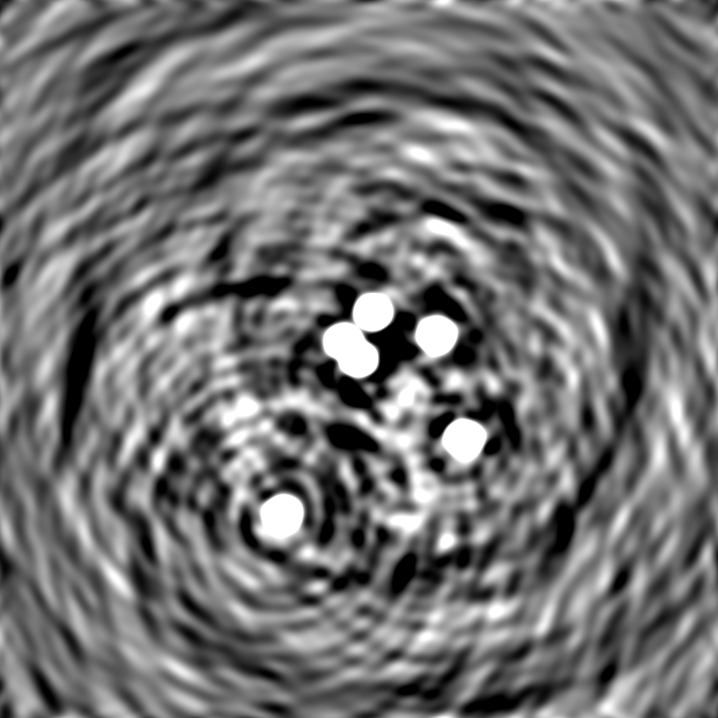
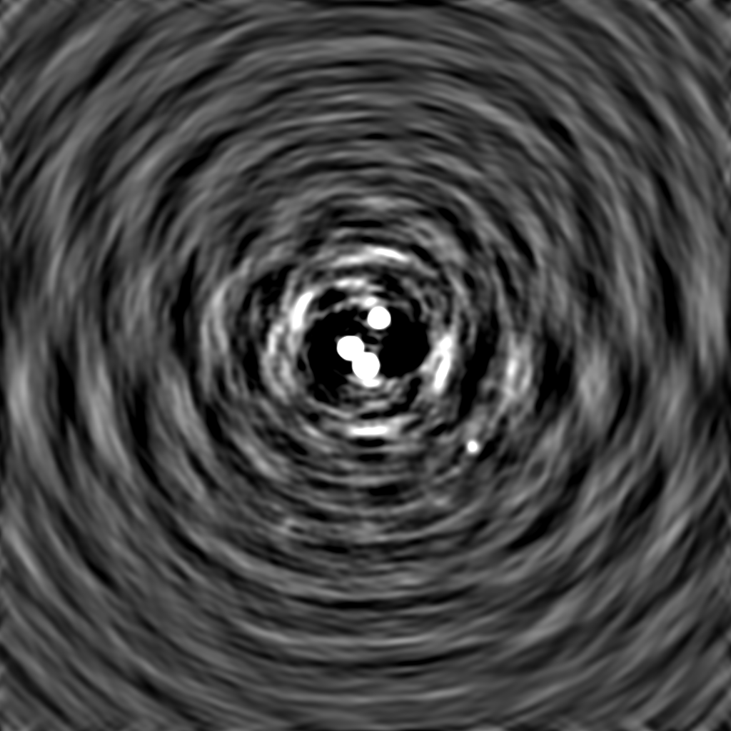
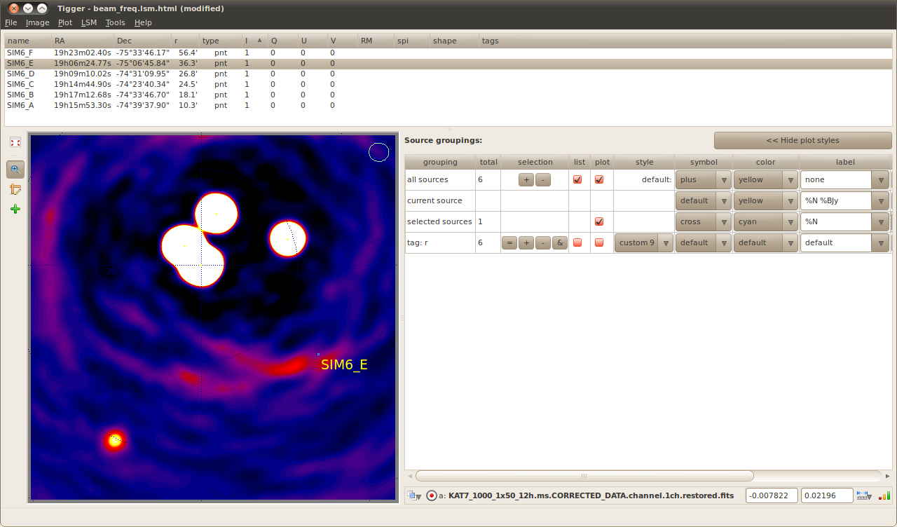
Once this has been successful, pop up the 'TDL Exec' menu again and make a cleaned image. The reason we're cleaning these images is that for sources that get attenuated away from the beam centre, you may find them being rendered invisible due to the strength of the sidelobes associated with the brightest sources in the field. You should be able to see, even in the thumbnail below, the attenuation effects of the beam.

In fact, it looks like source SIM6_E has completely vanished. Did we forget something? I don't think we did, so where has it gone?

You can load the FITS image up together with the sky model to examine its precise position as I have done in the screenshot below. If you saved the intrinsic FITS image under a different name then you can also play around with image differencing.

Anyway, that's one frequency channel. One final thing before we deal with the other five is to open the 'TDL Exec' menu (or the compile time options) and save the profile under 'source_colourization_apparent'. Again a standalone .tdl.conf profile for this simulation is provided in the data products below.

We've got the Measurement Sets, the sky model and the FITS beams so we could just repeat the above simulations for the next five frequency channels by hand. It'll be a lot easier to just script them though.

MeqTrees is perfectly happy to operate in 'headless' mode or batch mode, i.e. you can run it directly from the command line. This makes it highly scriptable, and this feature is basically essential for large calibration jobs. The software that makes the images from within the Meqbrowser is also a standalone command line tool called lwimager (based on the CASA imaging libraries) so we can script that too.

Before we begin however, the imager can sometimes grumble if appropriate columns aren't added to the MS, and in previous batch mode simulations for some reason this error pops up whereas it doesn't if we run a sim from the browser. It's easily avoided though. Attached below is a tiny Python script called add_imager_cols.py (courtesy of Tony Willis) that invokes a Pyrap function to do this task.

Before we proceed, pay your terminal a visit and in the folder that contains our Measurement Sets, run this script on all of them via:

for f in *.ms ; do python add_imager_cols.py $f; done

Now we're ready to proceed.

The plan here is to invoke both MeqTrees and lwimager from a script in order to do the following steps:

1) Simulate the intrinsic sky.

2) Make a cleaned image of the intrinsic sky and write it to a FITS file with a *.intrinsic.fits suffix.

3) Apply the beam patterns to simulate the apparent sky.

4) Make a cleaned image of the apparent sky and write it to a FITS file with a *.apparent.fits suffix.

There is a very handy script that runs batch jobs called meqtree-pipeliner.py, which should be in your path. If you run

meqtree-pipeliner.py -h

from the terminal you should get a bit of info about it. Essentially you provide it with a .tdl.conf file, a TDL script and the name of the TDL job you want it to run and it sets up a meqserver and executes the job. The real flexibility emerges when you realise you can tweak the input parameters between specificying the .tdl.conf file and the TDL script. We have an obvious use case for it in this simulation: in step (1) above we want to run the same simulation job on a series of Measurement Sets, and in point (3) above we need to do the same task, plus apply the appropriate simulated beam pattern.

I have attached a Python script (batch_beam_sim.py) which will hopefully perform steps 1 - 4 for you for all six Measurement Sets, including the one we just did by hand. The script is heavily annotated so you are encouraged to open it up and take a look inside and figure out what it's doing. I'm not the neatest programmer in the world (even when it comes to Python, I never let anyone see my Perl scripts), for which I apologize. I'm sure I'm not the most efficient either, so if you see something that can be done better please do implement it and send me your version. You might also want to investigate the --mt switch for meqtree-pipeliner.py if you are running this on a powerful machine.

Here's an example of one of the meqtree-pipeliner.py invocations from the script:

meqtree-pipeliner.py -c tdlconf.profiles \[source_colourization_apparent\] ms_sel.msname=KAT7_1000_1x50_12h.ms pybeams_fits.filename_pattern=beam_patterns/fitsbeam_L1000_$(xy)_$(realimag).fits turbo-sim.py =_tdl_job_1_simulate_MS

This loads the TDL parameters from tdlconf.profiles (also attached), specifically those from the [source_colourization_apparent] section. Following this, it changes the ms_sel_msname and pybeams_fits.filename_pattern parameters to the ones that the batch_beam_sim.py script has generated for that particular iteration. Finally it passes these parameters to turbo-sim.py and run the '1 simulate MS' job that we're now familiar with from the browser.

If you put the batch_beam_sim.py script in the same folder as your Measurement Sets and run it it should spend a minute or two running the simulations and generating the images for you.

It's debateable in our example which one is faster, doing this by hand or spending the time writing this script, but if you're still not convinced of the awesome power of batch mode then tonight's homework is to repeat this simulation for a thousand channels.

I'm not going to explain the ins and outs of the lwimager software. If you look up the CASA 'clean' task online or in the cookbook it should explain most of the parameters that you have access to with lwimager ('lwimager -h' is your friend here).

If all is well you should end up with the following in your terminal:

Finished!

I have made the following products:

KAT7_1000_1x50_12h.ms:

KAT7_1000_1x50_12h.ms.intrinsic.fits

KAT7_1000_1x50_12h.ms.apparent.fits

KAT7_1200_1x50_12h.ms:

KAT7_1200_1x50_12h.ms.intrinsic.fits

KAT7_1200_1x50_12h.ms.apparent.fits

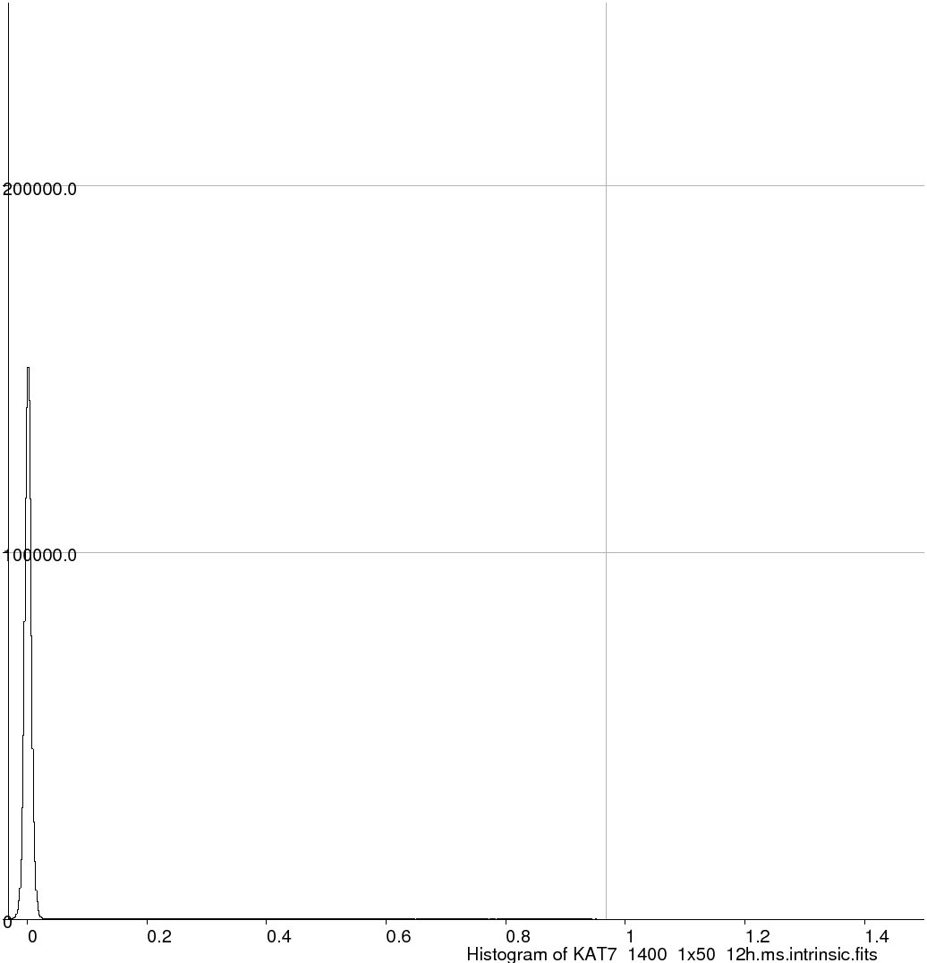
KAT7_1400_1x50_12h.ms:

KAT7_1400_1x50_12h.ms.intrinsic.fits

KAT7_1400_1x50_12h.ms.apparent.fits

KAT7_1600_1x50_12h.ms:

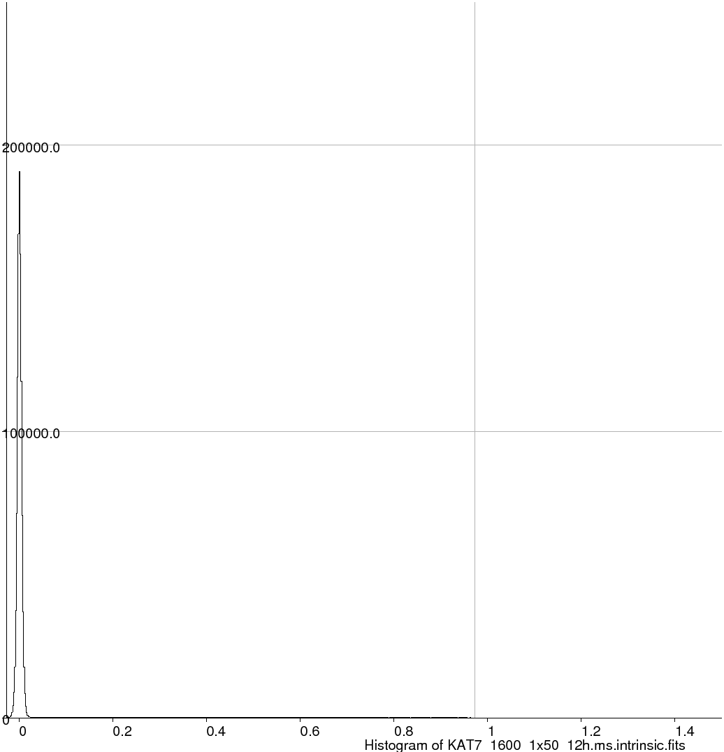
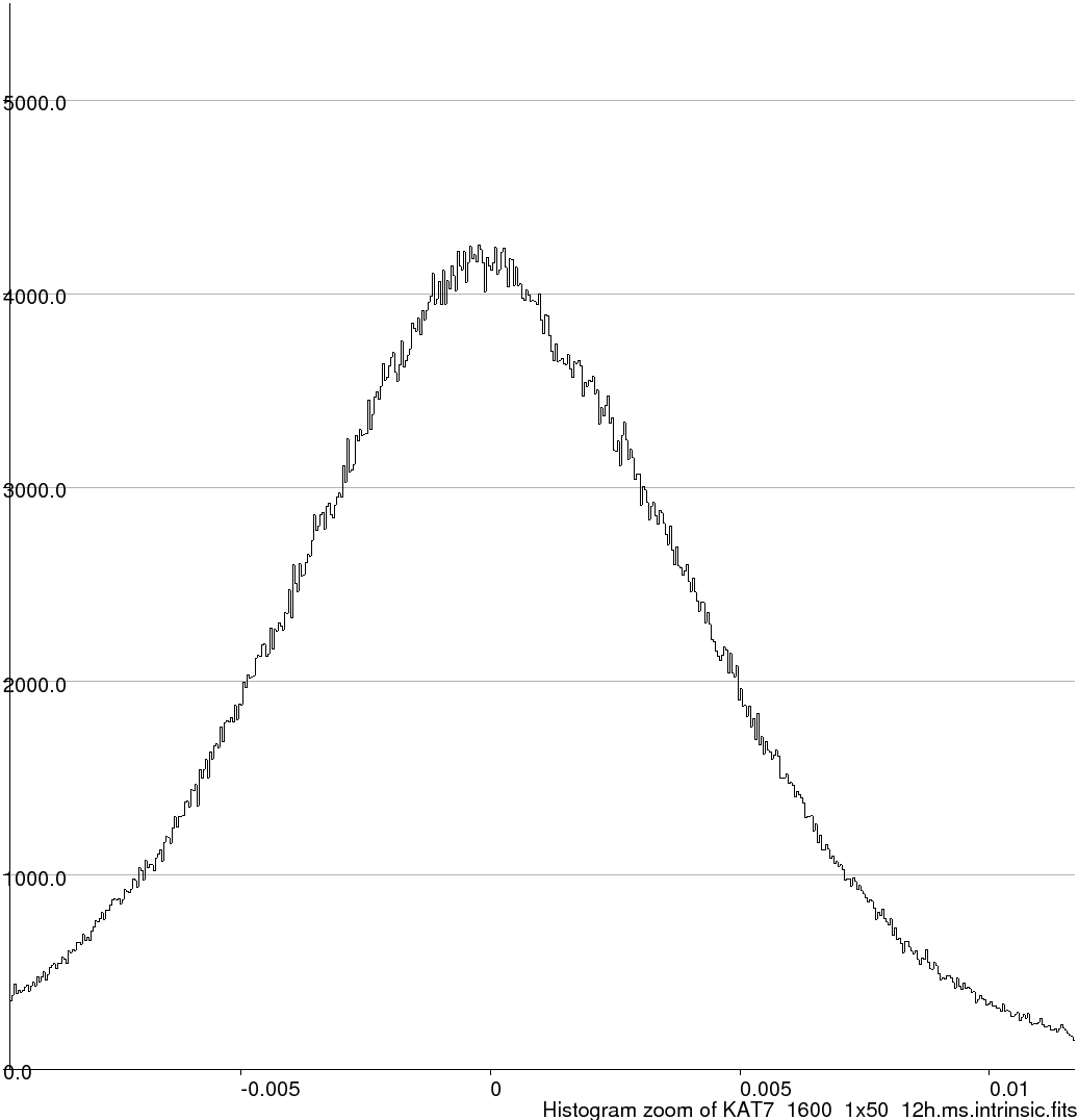
KAT7_1600_1x50_12h.ms.intrinsic.fits

KAT7_1600_1x50_12h.ms.apparent.fits

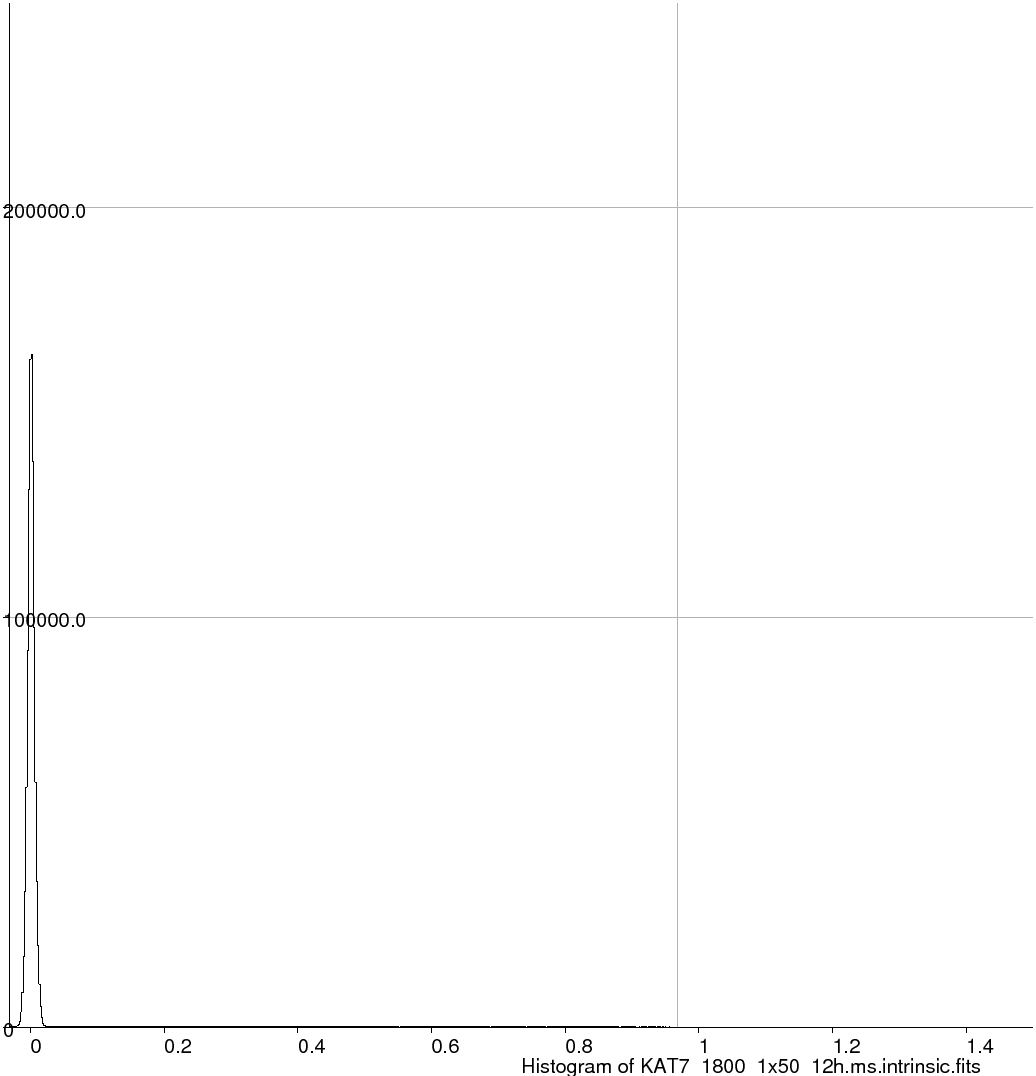
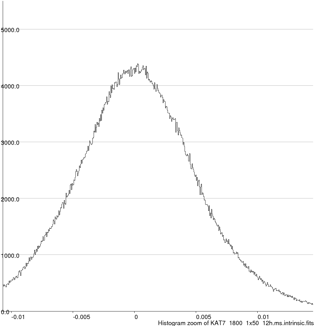
KAT7_1800_1x50_12h.ms:

KAT7_1800_1x50_12h.ms.intrinsic.fits

KAT7_1800_1x50_12h.ms.apparent.fits

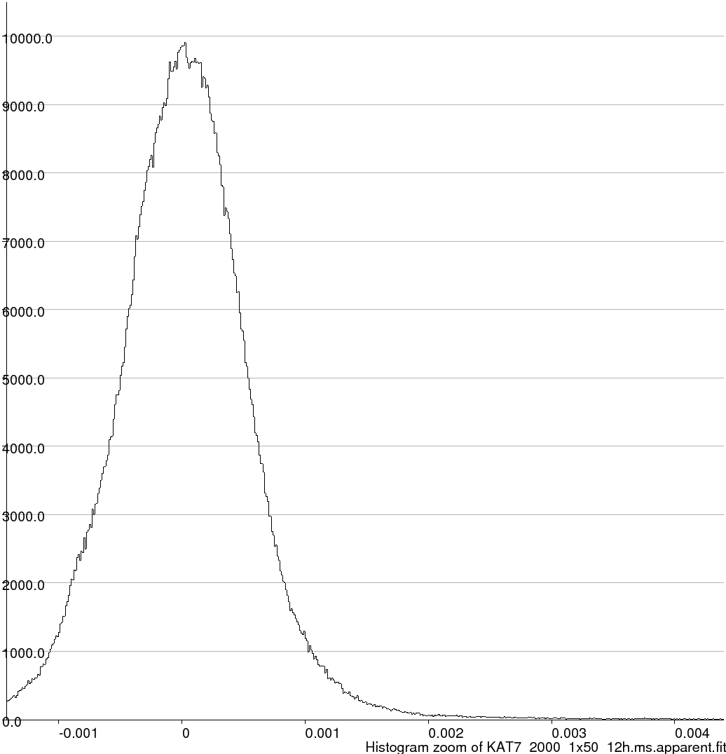
KAT7_2000_1x50_12h.ms:

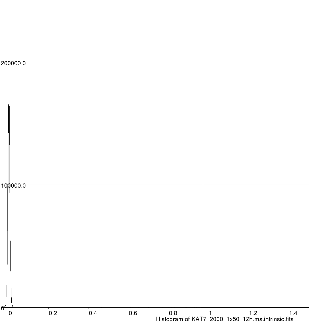
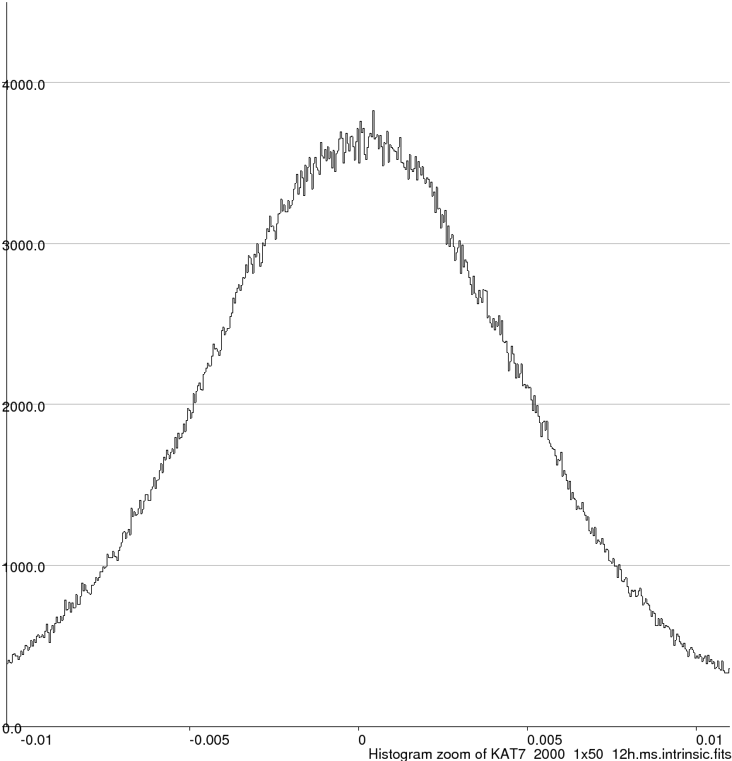
KAT7_2000_1x50_12h.ms.intrinsic.fits

KAT7_2000_1x50_12h.ms.apparent.fits

When the script proudly proclaims that "I have made the following products" what it should really say is "I have made a load of data products, and of those the following are the ones you want to keep".

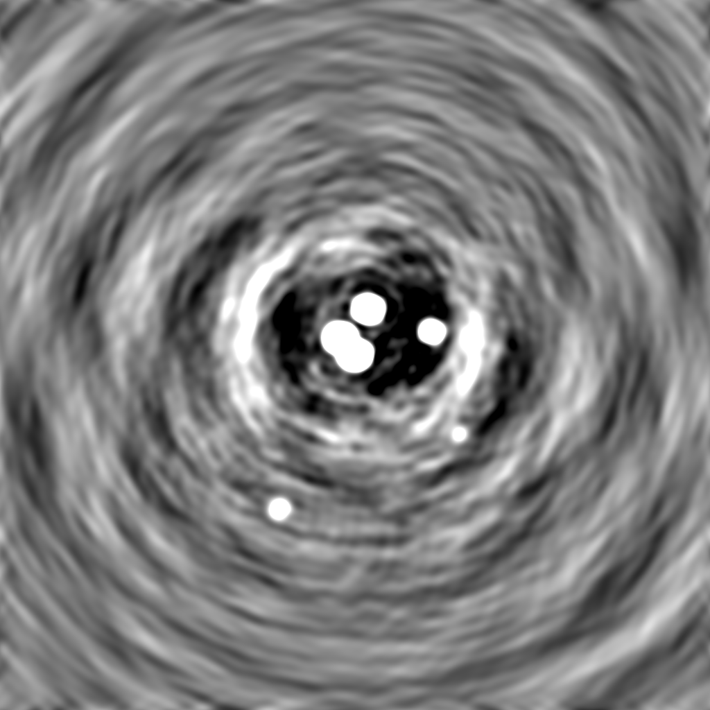
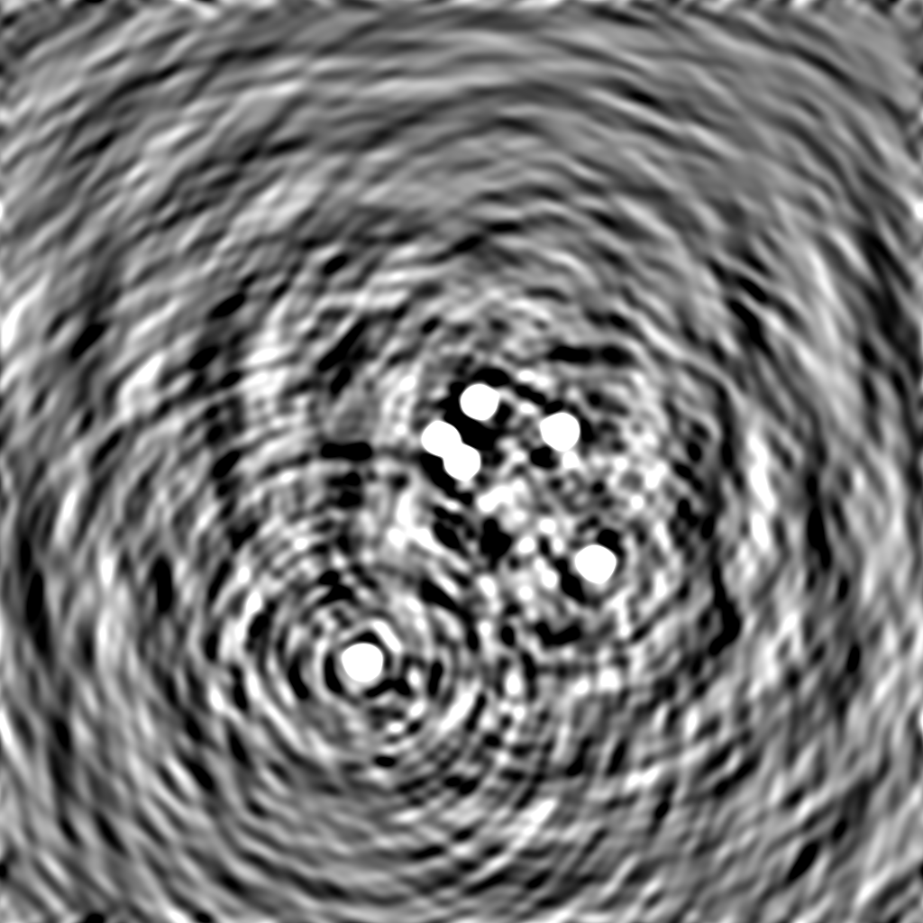
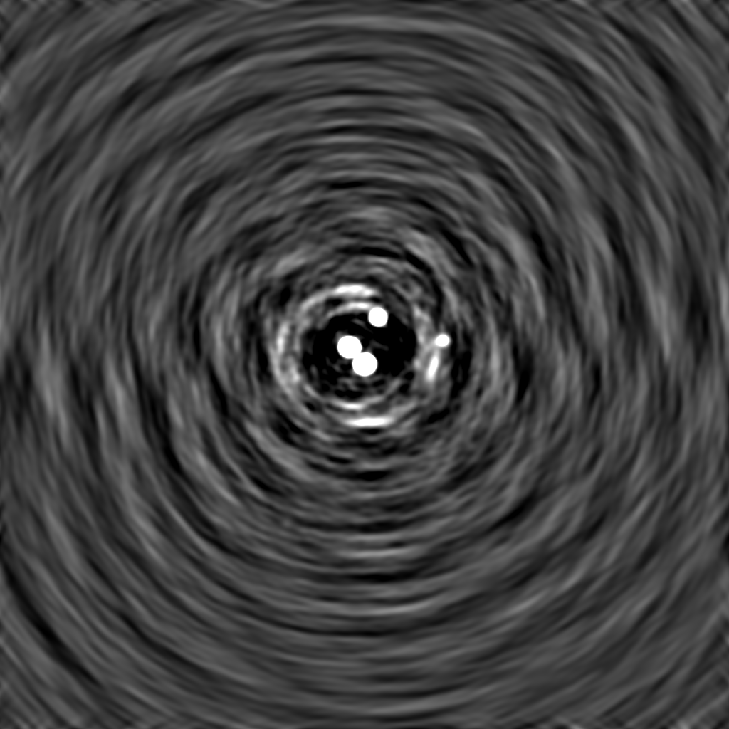
The deconvolution process results in a few data products that are surplus to our requirements at this point, and we can basically delete anything that has a *.model, *.residual or *.restored suffix. The images that we want to keep are *.apparent.fits and *.intrinsic.fits, i.e. the FITS images that are attached and rendered below.

(There's probably a way you can tweak the lwimager command in the script in order to prevent the surplus images being kept in the first place...)

By "source colourization" what I really mean is "spectral corruption".

The six "intrinsic" FITS images we have above contain the true spectral shapes of six 1 Jy point sources. Since our sky model assumed a flat spectrum, these intrinsic spectra should be flat across our band.

The six "apparent" FITS images we generated similarly contain the apparent spectral shapes of the same six sources, and we can see how these have changed in the presence of solely primary beam effects. Get your predictions in now!

If you're so inclined you can open each of the FITS images, not down the brightnesses of each source and break out the graph paper. A slightly easier method is to just write a script. The script I've written to extract and plot the source spectra is attached below, with the blisteringly-imaginatve name 'plot_spectra.py'. Again this script is probably a little rough around the edges (IANA programmer) but it does the job. It's annotated again so please have a look inside.

Basically it uses the Tigger API (I refer you to the Tigger Users' Guide for a full description) to get the positions of the sources in our sky model. It then uses Pyfits and the world coordinate system info from the FITS headers to locate the pixel positions of each source in the map. It extracts the brightness at the relevant position from each of the spectral channels for both the true and apparent case and then plots a per source spectrum using matplotlib which is saved to a file.

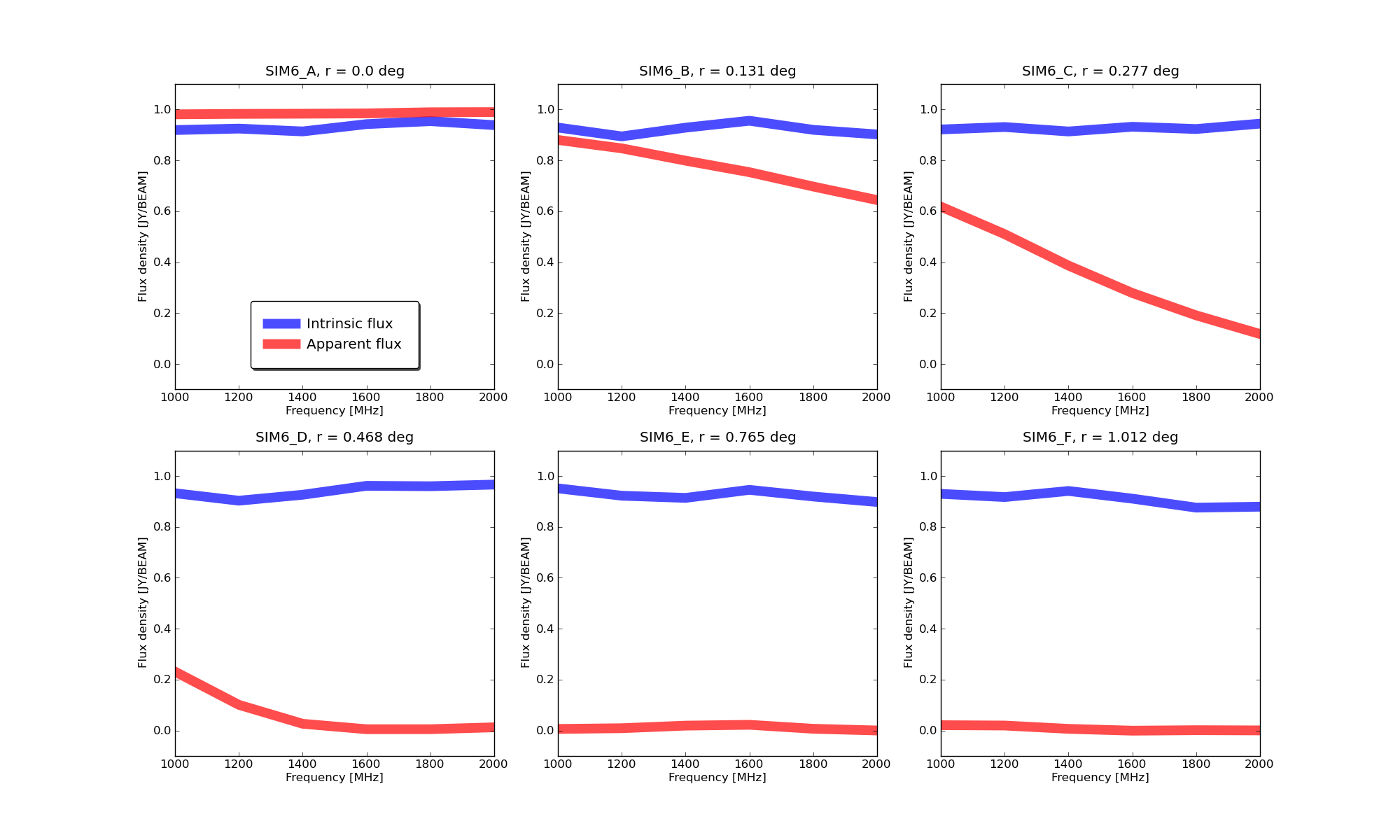
The spectra of each source are plotted and attached below. Each panel represents one source. The blue line shows the measured true source spectrum. This should be a flat line at 1 Jy, as per our sky model. The red lines show the apparent measured spectrum of the source due to the beam effects. As you can see, as well as the beam attenuation, the spectral shapes of the sources can go from flat to convex (SIM6_B) or to concave (SIM6_C, SIM6_D) for sources in the main lobe. The main lobe shrinks with increasing frequency so a source at a fixed distance from the phase centre is observed with reduced sensitivity, causing the attenuation to increase as we move towards the top end of the band.

Sorurce SIM6_E is an interesting case in that it actually rises and then falls as we move up through the band (find and edit the ylim parameter in the plotting script if you want a better look). This is due to a sldelobe washing over it as the observing frequency varies. It also explains why this source was completely attenuated in our first 'by-hand' simulation, as for the 1 GHz observation is was sitting in a primary beam null and was basically invisible to the instrument.

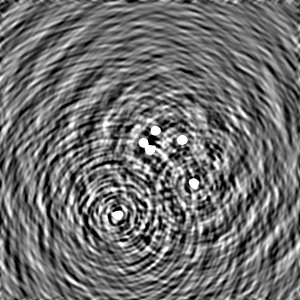
What is causing the ripples in the intrinsic spectra, and why are these sources attenuated? Well, in my opinion this boils down to the PSF and incomplete deconvolution. The PSF is also frequency dependent and sidelobes from one source wash over the other. We weren't particularly careful in our deconvolution so some sidelobes remain, as can be seen in the FITS renders with the compressed pixel scales in the previous Purr entry.

Of course now that you are a batch mode master you can repeat this simulation such that it only simulates and images a sky that only contains each source in turn, to see if you can get the blue lines to match what we know the true sky to be. (Will you need to do deconvolution?)