SSSC1 and the Calico WSRT scripts

This log will guide you through some of the things you can do with one of the SSSC Measurement Sets and some pre-existing TDL scripts. If you've installed MeqTrees then you should find the Calico framework within the Cattery. This contains a bunch of pre-existing TDL scripts primarily designed for the calibration of data from the Westerbork Synthesis Radio Telescope (WSRT).

First we'll (1) have a look at the data the Measurement Set contains, then (2) we'll make an image. After that we'll (3) look at source subtraction and then finally (4) do some calibration.

Fire up the MeqBrowser and open Cattery/Calico/calico-view-ms.py. This script is intended for a first-look at any Measurement Set you might have. It's not WSRT-specific; you can examine anything with it (in my experience).

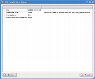
The first thing you'll be presented with are the compile-time options. There's not much to do here other than point it at the Measurement Set. If you wish you can tell it to only examine a subset of antennas (it defaults to all of them), and you can also select correlation products, the default being all four.

It should all be self-explanatory, but there's a screen shot below.

Hit compile and it should build a small tree and bring up the runtime options.

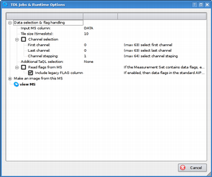
The runtime options window contains further options for data selection.

For calibration purposes Measurement Sets typically have three columns, DATA, CORRECTED_DATA and MODEL_DATA. You can select which one of these you'd like to examine (the simulated Measurement Sets should only have something in DATA).

The tile size tells MeqTrees how many timeslots to digest at once. Visibility data are processed in time/frequency 'tiles', the default shape of these includes all frequency channels and a number of time slots specified by the value in the options.

You can select a range of frequency channels with the next option.

Finally you can ask MeqTrees to read in any information about bad data which have been flagged out, if the Measurement Set contains such a table. These simulations don't, so this can be left deactivated.

Ignore the 'make an image' option for now, we'll come to that in a little while.

Don't click 'view MS' just yet, though.

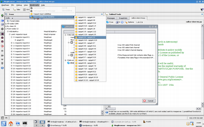
Before we view the MS we have to load a few bookmarks. These are pre-defined in the TDL script to allow visualisation of certain nodes in the tree.

With the runtime options window still open you can select these from the bookmarks menu (see screen grab below).

Select 'inspect input visibilities' and one of the 'by baseline' options, then select 'view MS'. If you've closed the runtime options window by mistake then just click the 'TDL Exec' button in the toolbar.

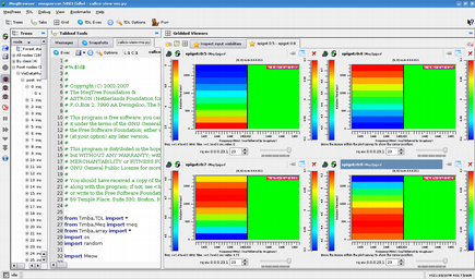
You should see a few plots appearing in the 'Gridded Viewers' section. The 'viewers' screen grab below shows the 'by baseline' results.

What you can see here are the amplitude (left) and phase (right) as a function of time (y-axis) and frequency (x-axis), with the colour scale indicating the value.

Note how the phases are completely flat. This is consistent with a single point source at the phase centre. The variation in the amplitudes is due to the random antenna based gain errors we included. Of course, we have the benefit of knowing exactly what went into the simulation here, but examining visibilities in this way can tell you a lot about the source structure without making an image.

This is a good habit to get into.

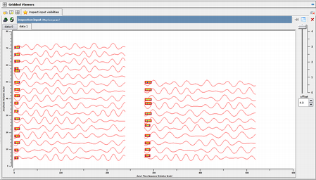
If you click the 'inspect input visibilities' tab you will see the amplitude versus time for each baseline, also shown below in the 'inspector' screen shot. If you right-click on the plot you can choose phases with the 'complex data selection' option. You can also zoom by drawing boxes. If you middle click on one of the plots it will pop out into a separate window.

Just play around, you'll get the hang of it.

Let's make an image. If you've read any of the PURR logs which (loosely) describe the generation of a the simulated Measurement Sets you might already be familiar with this part.

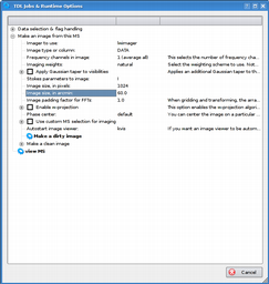
Click the TDL Exec button again and expand the 'Make an image from this MS' menu.

Imaging is handled by software external to MeqTrees, but invoked by the Browser. This will probably be the lightweight imager (lwimager) from casarest, or the imager from that much-maligned and misunderstood butt of all radio astronomy jokes, AIPS++.

The imaging options are set up via the Browser and then passed to the imager in the background. Once its generated the FITS file it should also automatically invoke the specified viewer.

An example set of options is provided in the data products below.

Once you've set them up just click 'Make a dirty image'.

You'll also notice there is the facility to CLEAN the image (i.e. deconvolve the PSF). Once curiosity of the lwimager is that it doesn't seem to want to clean the DATA column of a Measurement Set, so this feature is out of our reach for now...

What you can see below is the dirty image, basically the central point source convolved with the PSF of the Westerbork Array. If you look closely you should be able to see some radial features, reminiscent of the waves in Saturns rings. This is another by-product of the varying receiver gains, an unwanted artefact which we should be able to remove with a bit of calibration.

The 'histogram' is also a very useful plot. It shows pixel counts as a function of brightness. The story that this one tells is that there are a large number of low brightness pixels and a few of very high brightness. The y-axis scaling is normalised when PURR automatically generates the figures, so the high brightness ones barely register, although you should be able to see the blue line hugging the x-axis.

Restart the MeqBrowser and load the Cattery/Calico/calico-wsrt.py TDL script. The compile time windows should pop up. There are a truck-load of options here, mainly for solving for different Jones matrices. We're working on a very simple simulated Measurement Set though, so we'll only use a couple of the options.

Please note that this document is a not an exhaustive description of this TSL script. A deeper explanation of the options available here can be found in the 3C147 calibration tutorial on the MeqWiki.

The first thing we'll do with this script is use it to subtract the source and then examine what's left.

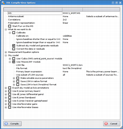
If you have already selected the Measurement Set then expand the 'What we want to do' and the 'Sky model' menus, and set the options up as shown below.

The first three tick boxes tell us that we're not doing any calibration at this stage. We're going to subtract the source from the visibilities, and finally since no calibration has taken place there will be no need to correct the remaining residual visibilities.

As for the sky model: we know that this Measurement Set contains a central point source as this is all we included in the simulation. For the calibration of real data things obviously aren't this simple, and construction of a sky model is an iterative process that must be done with great care, even with prior knowledge of your targets.

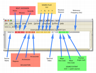
We're just introducing concepts here though, so let's pretend we're omnipotent. Select the 'Use 'MeowLSM' module' option. LSM files come in many flavours but the one to use here is the same one we used to specify the simulation. This is included below, together with a diagram poached from another PURR log which explains the columns.

Obviously there's a tick missing from the screen grab below, and that's the one that activates PURR.

Once this is all set up then hit compile.

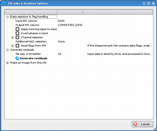
Examine the runtime options menu below.

What this tells us is that we're sticking spigots in the DATA column to read the data, subtracting the visibilities that correspond to our source model, and then putting sinks in the CORRECTED_DATA column to write it. Nothing fancy is going on here, we're not limiting the channel selection or reading any flags.

Click the 'generate residuals' button when you're ready.

Once this has finished we can image the residuals. Click the 'TDL Exec' button and expand the 'Make an image from this MS' menu.

A critical option here is that we image the CORRECTED_DATA column, as this is where MeqTrees wrote the source-subtracted visibilities. The original DATA column will be left untouched.

Average all the channels, and let's image our usual 30 arcminute field. Click 'make a dirty image' and it should return something similar to the file in the data products below.

What are we seeing here?

Remember when this simulation was generated we added the slowly varying receiver gain errors. The residual structure here is the result of these errors, and you can see the levels at which this pollutes the map in the histogram. All we have done so far is subtract a model visibility set consistent with a 10 Jy unpolarized source at the field centre.

A more sensible thing to do is to do some calibration and try to solve for those receiver gain errors.

This section describes the first proper calibration step.

Click the 'TDL Options' button again and this will bring up the compile-time menu. Everything should be as it was for the previous step. We want to do some calibration now so expand the 'What we want to do' menu, check 'Calibrate' and make sure we're calibrating on visibilities. Enable 'subtract sky model' and 'correct the data or residuals'.

This time we'll also solve for the values of a 2x2 gain matrix, the so-called G-Jones matrix. Select the 'Use G-Jones (receiver gains/phases)' option, and check the 'Use FullRealImag module' box. This solves for the real and imaginary parts of this matrix simultaneously.

Click compile and it will build a tree.

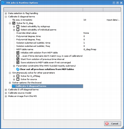
Examine the run-time options below. The tile size is still set at ten, but we're also setting the solution sub-interval (sub-tile) for time to 1 and leaving frequency as 'none'. You can use this to set the number of solutions per tile, e.g. setting both to 1 would result in one solution per time and frequency point. We know that the gains are stable in frequency and variable with time, hence these values. One solution per time slot is more computationally expensive but it's also more accurate.

Don't forget about bookmarks!

When you're ready, open a bookmark or two: 'inspector G' and the residuals are always useful.

If you wish you can also perform solutions for the off-diagonal terms of the G-Jones matrix, either subsequently or simultaneously.

Click the 'Calibrate G diagonal terms' button and examine the 'inspector G' bookmark to see your gain solutions.

Open the 'TDL Exec' menu again. It should remember how we like our images, but double check anyway. Expand the 'make an image from this MS' menu, make sure we're imaging the CORRECTED_DATA channel which now contains residual visibilities, i.e.what's left after we've subtracted the source and corrupted the data with the G-Jones.

Click 'make a dirty image' and you should end up with something like the image below.

The image due to the residual calibration errors has noise-like emission on the nano-Jansky level. Of course this is an idealised simulation which does not contain the thermal noise which pervades all real observations, does not contain numerous or complex radio sources, and is also free from all but the simplest of data corruptions. Nonetheless the techniques we have employed to arrive at this image are fundamental, and all calibration is basically an extension of these ideas.