SSSC25_WSRT.MS

As well as the usual +/- 20% slow variation in the receiver gains SSSC25 also introduces a frequency dependence on the gains to simulate a simple bandpass shape.

This Measurement Set requires a pair of TDL scripts external to the Siamese Framework. These are the BJones module which simulates the simple bandpass shape (simplebandpass.py) and the modified example-sim-bjones.py which factors this module into the simulator.

These are added below. If you want to try these out for yourself you'll have to run the Meqbrowser from the folder where these scripts reside. Have a look at simplebandpass.py and see if you can figure out what shape the bandpass will be.

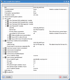
Examine the compile-time options below. As you can see this simulation is much the same as SSSC1, but you'll notice the addtional 'Use B Jones' option which is checked.

The sky model is the same as SSSC1: a 10 Jy point source in the centre of the field. You may also notice the 'Error model for slope' option, but we'll leave this for a subsequent simulation.

Hit compile to build the tree.

The runtime options should pop up but before you click 'simulate MS' we'll open a viewer to examine the bandpass.

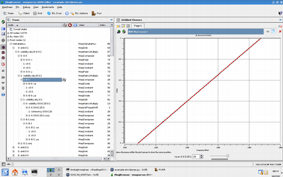
Cancel the runtime options window and expand the tree from the root nodes. Referring to the screen grab below will help.

Find the sink corresponding to baseline 0:1 and keep expanding it. You should be able to see the visibility generated by this baseline for source SSSC25 furthest down (or up) this branch of the tree, and see the hierarchy of operations, in this case the simulated B- and G-Jones antenna-based corruptions.

A nice feature of MeqTrees is that you can visualise any node in the tree. You might have read how to do this elsewhere but here it is again:

We want to examine the bandpass so right click the B:0 node and select publish. You should see a little newspaper-type icon appear next to it. Right click again and select 'new display with' and then 'results plotter' from the sub menu.

A blank viewer should spring up, ready to be filled with the values as they come in when the tree is executed. The Meqbrowser is intelligent here in that it examines the structure of the node and generates a suitable plot without you having to think about it.

Press the 'TDL Exec' switch again, make sure the 'output column' is set to 'DATA' and click 'simulate MS'.

You should then see a plot resembling the one in the screen grab below. A couple of things to note:

1) What we've done is put a simple gain slope across the bandpass. If you're short of something to do then you could try calibrating this using the B-Jones option in the WSRT Calico scripts. Remember we're omnipotent for the open challenges and we know for certain that we have a spectrally flat 10 Jy point source at the phase centre.

2) You can see from the tree that the B- and G-Jones are antenna based. Note how the conjugate point has B and G operations corresponding to the second antenna index in the baseline pair. You could re-write the bandpass TDL code if you wanted to simulate a different bandpass for each receiver.

Once the simulated visibilities are written then we can make an image. Click the TDL Exec button and expand the imaging options. As usual we're imaging the DATA column (which should be the only column that contains anything), averaging all the channels and imaging a 30 x 30 arcminute region.

Click 'make a dirty image' and it should return something like the image below.

Another nice way to see the effect is to image all the channels and perform no averaging. If you do this with 1024 x 1024 pixel frames then the FITS file is 257 MB which I don't really want to add to the PURR log, so there's an AVI available in the data products below.