SSSC30_WSRT.MS

Let's use the five-source sky generated for SSSC21 and perform a primary beam simulation. The primary beam of an interferometer at its most benign will attenuate the brightness of sources away from the pointing centre. For an array consisting of equal dishes (e.g. WSRT, VLA) the primary beam of the interferometer closely resembles the of a single element. For a heterogeneous array (e.g. eMERLIN) the situation is a lot more complicated, and even more so for interferometers whose elements are phased arrays (e.g. LOFAR).

Furthermore the primary beam response, characterised by the so-called E-Jones matrix, generally exhibits time- and frequency-dependence and has different properties per polarization. Accurate understanding of it is essential if you want to achieve high dynamic range over a wide field. Fortunately the WSRT E-Jones is well behaved and well understood, so we're in at the shallow end here.

Please take a look at SSSC21 for to see what the sky in this simulation would look like without the primary beam effects. The note about intrinsic and apparent fluxes in SSSC20 might be worth reading, and in any case you should have a read about primary beams in a synthesis imaging text book if you're serious about them. This PURR log won't be an exhaustive introduction by any stretch of the imagination.

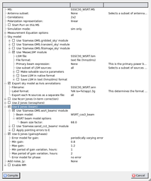
As usual, point the MeowLSM module at the LSM file (this one is the same as SSSC21). Remember to write out the annotation file, as this will be particularly useful for this exercise.

If you examine the screen shot below, you'll see that everything else is business-as-usual, except we've also checked the 'Use E Jones (beam)' module, and the 'Use Siamese.OMS.wsrt_beams' sub-option.

The WSRT voltage beam can be accurately modelled using a cos-cubed function with some scaling factors thrown in (see the WSRT, or NEWSTAR users guide for more info).

Click 'compile' to build the tree.

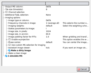
Once the runtime menu appears, make sure the 'Output MS column' is set to 'DATA' and click 'simulate MS'. Once this is done, click the 'TDL Exec' button and make an image. You should be able to see that the central source retains its true brightness while the off-axis sources have been attenuated. Overlay the annotation file (attached below) for additional clarity.

A very nice feature of example-sim.py (and MeqTrees in general) is the ability to stick a spigot into one column of the Measurement Set and subtract your predicted data from the existing data, writing the difference to another column of the MS. You will have already encountered this technique if you have read the 'SSSC1 and Calico' PURR log, but it's also very useful for simulation.

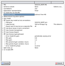
In this exercise we'll disable the E-Jones matrix, predict the visibilities and subtract them from the DATA column, which contains visibilities which were generated with the primary beam simulation included.

Click the 'TDL Options' button to bring up the compile time menu. DIsable the 'Use E Jones' option, and set 'Simulation mode:' to 'subtract from MS'. Click compile.

[If you examine the tree at this point you should hopefully see both spigots and sinks under the VisDataMux node.] S For the run time options make sure 'Input MS column' is set to 'DATA', and we'll write the differenced visibilities to the 'CORRECTED_DATA' column. Set up these options and click 'simulate MS'.

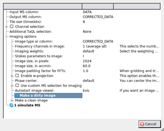
Imaging set up is as before, but the image is derived from the 'CORRECTED_DATA' column. The result shown below represents the net image plane effect of the E-Jones matrix for the WSRT. Note that the largest negatives are the ones furthest away from the pointing centre in a radial sense. The central source also leaves no mark because the gain in this direction is unity with and without the simulated primary beam.

This technique is very powerful for determining the levels at which various corruptions affect your final image.

1) Run it through the Calico-WSRT scripts with an eye on the E-Jones options

2) Try to derive a sky model based on the apparent fluxes of the sources and use that for calibration (c.f. self-calibration)

3) Make your own differential simulation to gauge the effects of pointing errors (these are incorporated into the E-Jones by shifting the response pattern on the sky).