SSSC

Spigot2Sink

The spigot2sink (s2s) diagrams shown here are your indispensible guide to how the SSSC Open Challenges are put together, and to what we ask you to do with them.

First of all, do not be intimidated by the jargon, like "uv-data" or "Jones matrices". It is really quite simple, and people who are productive in writing software (and thus have organized brains) will quickly pick it up. In the meantime, you should be able to get along with the brief explainations at the bottom.

Page contents (click an entry to scroll down to that section):

1. Inspecting uv-data
2. Generating simulated uv-data
3. Solving for M.E. parameters
4. Subtracting the LSM sources from the uv-data
5. Correcting the uv-data
6. The full Monty
Appendix

1. Inspecting uv-data

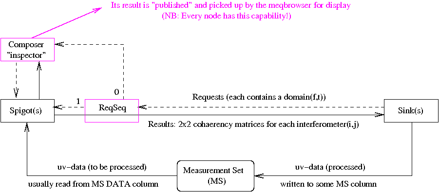
Figure 1 (click to enlarge)

Fig 1 shows the simplest operation of all: inspecting the uv-data in a given Measurement Set (MS). The latter is the uv-data file of the CASA/AIPS++ package. Converters exist to and from the data-formats of the other major packages (AIPS, MIRIAD, NEWSTAR). In this section, we show the basics of MeqTree visualization. This is already impressive but, with your help, we aim to offer many more ways to look at uv-data and its associated meta-data. In the meantime, you should also look at what CASA/AIPS++ has to offer in MS visualization.

The calico-view-ms.py TDL script, bundled with the Calico Framework within the MeqTrees Cattery, is for examining uv-data. It might be useful to examine the nodes that this script generates in parallel with reading this text. Brief instructions for its use can be found in the PURR logs for open challenge 1.

Note that the schematic tree that is shown in fig 1 (and in all subsequent block diagrams) should be interpreted as N(N-1)/2 parallel subtrees, one for each interferometer(i,j) in an N-station array. Each interferometer has its own MeqSpigot node (which reads its uv-data, usually from the DATA column of he MS) and its own MeqSink node (which writes the processed uv-data back, usually into another column of the MS).

By default, MeqTrees steps through the uv-data in time order. A single "VisDataMux" node generates a succession of processing Requests, which are issued to all MeqSink nodes simultaneously. Each Request contains a "domain", i.e. a rectangle in freq-time space. Successive Requests usually have domains that span all the freq channels in a "spectral window", but only a limited number of "time-slots" (e.g. 10 minutes). As you probably have grasped by now, all the nodes in a tree have the same simple task: to return a Result that contains values for the cells of the requested domain.

If fig 1, the flow of Requests is indicated as dashed arrows, while the flow of Results is in solid arrows. In later block diagrams, the Request flows will be omitted to avoid clutter.

The uv-data may be visualized in two ways. First of all, EVERY node in a tree, however complex, has the capability to "publish" its Results, which are then picked up by the browser for display. Thus, you have access to every intermediate result during every stage of the processing. The PURR log in the first Open Challenge explains how to deal with this embarassment of riches.

Secondly, the Resuts of an arbitrary collection of nodes may be visualized together in the same plot. This is a feature of the MeqComposer node (Its main function, which will not be discussed here, is to put the Results of its child nodes into a single "tensor" Result). The Request for this "inspector" node is generated with the help of the MeqReqSeq (request sequencer) node shown in fig 1. Rather than issuing its Request to all its children simultaneously, it does so in a user-defined sequence (indicated with 0 and 1 here). For each child, it waits for it to return a Result before issuing its Request to the next child. When finished, it passes on the Result of a user-defined child (in this case the MeqSpigot).

2. Generating simulated uv-data

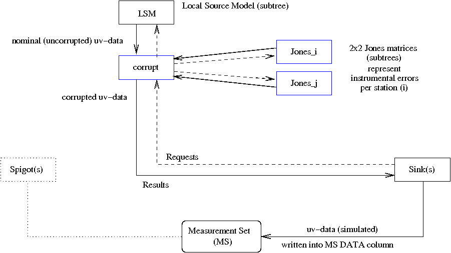
Figure 2 (click to enlarge)

Fig 2 shows how simulated uv-data are generated. The uv-data for the various Open Challenges have all been made in this way. For each challenge, the TDL script that generated the data is available for scrutiny. It is highly recommended to read the Python code, and to browse the resulting tree in the meqbrowser. It goes without saying that you should also read the PURR log, of course.

The generating TDL script may also be cannibalized by the more ambitious among you, e.g. to generate new challenges.

As before, the schematic tree in fig 2 represents N(N-1)/2 parallel subtrees, for all interferometers(i,j). The flow of Requests is indicated once more as dashed arrows. The spigots are indicated for cintinuity with the other figures, but they are not needed for simulation, of course.

As described in the PURR log, an empty MS should be generated by an AIPS++ utility called "makeMS". This is done for a particular telescope (e.g. WSRT, or VLA), with a given station configuration, and a given number of time-slots and freq channels. It also specifies a pointing centre in the sky.

A sequence of processing Requests is generated, for contiguous time domains (usually 20 minutes or so). Larger domains are more efficient, but the maximum size is limited by the available memory.

For each Request, the Local Source Model (LSM) subtree calculates values(f,t) for the four Stokes parameters (I,Q,U,V) of each source. For each interferometer(i,j), and assuming linear polarization, these are converted into a 2x2 cohaerency matrix. For a point source in the field centre, the 4 (complex) elements are: XX=I+Q, XY=U+iV, YX=U-iV, YY=I-Q. The nominal (uncorrupted) uv-data are the sum of the contributions from all the sources in the LSM.

For each Request, the Jones matrix subtrees calculate the instrumental errors(f,t) for the various stations. The elements of each 2x2 Jones matrix are 4 complex numbers. The simplest case is the GJones matrix, which is a diagonal matrix that represents complex "station gains". The simulated instrumental errors (e.g. station phases or gains) are simply generated by means of small subtrees that generate sinusoidal errors with different periods in time and frequency.

NB: The GJones with its "antenna gains" is the staple of the 2GC data reduction packages, which do not use an explicit Measurement Equation (M.E.). MeqTrees does, and can handle Jones matrices that are themselves the product of a sequence of Jones matrices for different instrumental effects. The TDL script that is used here illustrates this by offering a small selection of Jones matrices, which are used for the various Open Challenges. As always, you are invited to play with this script, or even cannibilize it) to generate your own Open Challenges.

The simulated uv-data are simply the nominal visibilities calculated by the LSM subtrees, corrupted (by matrix multiplication) by the station-based instrumental errors calculated by the Jones matrix subtrees. Optionally, gaussian noise mey be added in this stage. The MeqSink nodes then store them in the DATA column of the MS.

3. Solving for M.E. parameters (MeqParms)

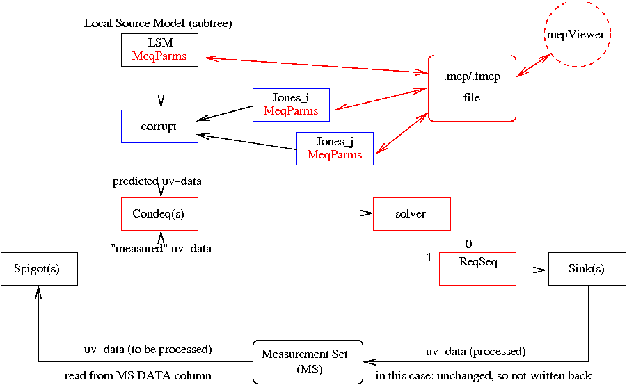
Figure 3 (click to enlarge)

Fig 3 shows how one may solve for (arbitrary subsets of) the M.E. parameters. Note that the LSM and Jones subtrees now contain MeqParm nodes, which are connected to a .mep or .fmep file to store their values for the different domains. (NB: An .fmep value is a more efficient version of a .mep file. Both are supported for the moment).

A viewer is being developed to scrutinize the stored MeqParm values, and even to manipulate them (e.g. smoothing). Unfortunately, this very useful tool is not compatible with our current release, but it will be with the one we plan for September (i.e. before we go to Nancay).

In this case, there is only a single MeqSolver node for the entire tree, i.e. for all N(N-1)/2 interferometer subtrees, which share the same LSM subtree(s), and N different Jones matrix subtrees. The solver node gets its Requests via a ReqSeq node in the same way as the inspector node in fig 1 (see also fig 4 and 5).

The solver solves for a user-defined subset of the M.E. parameters. These are made "solvable" by giving the solver a list of any subset of MeqParm nodes that are available in the Jones and/or LSM subtrees (note that instrumental and source parameters are treated equally here!).

The children of the solver are N(N-1)/2 MeqCondeq nodes, which supply it with "condition equations". A MeqCondeq has two children, which supply it with "predicted" and "measured" values (from the MS). The solver tries to minimize the difference between these two, for all MeqCondeqs simultaneously, in a Least Squares sense. Therefore, it is very instructive to visualize the MeqCondeq Results, for instance with an "inspector" node. Independent of the problem, the final MeqCondeq results should be noise-like. Obviously, this will only be the case if the solution has converged, and if one is solving for the correct M.E. and the correct subset of M.E. parameters(!). Dealing with this question is the core of what we are trying to achieve with MeqTrees.

The condition equations are accumulated in a solution matrix, which is then inverted to produce incremental improvements of the values of the solvable MeqParms. These are passed back up the tree to the relevant MeqParm nodes. The updated (and hopefully better) MeqParm values are then used in the next iteration. Since the M.E. is usually non-linear, multiple iterations will usually be needed before the solution is converged. This is controlled by the solver, and may be visualized in its Result in the usual way. (In the future, with your help, we plan to offer different solvers, and much more solver visualization).

4. Subtracting the LSM sources from the uv-data

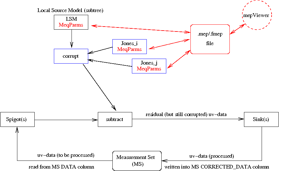
Figure 4 (click to enlarge)

Fig 4 shows how source contributions may be subtracted from the uv-data. Since, the data in the MS are corrupted with instrumental errors, we must corrupt the nominal source visibilities with the same errors before they are subtracted. In this case, we assume that the correct MeqParm values have been obtained somehow (e.g. by solving for them, or by transferring them from calibrator observations), and reside in the .mep/.fmep file.

Subtracting the contributions of known sources from the uv-data is one of the corner-stones of 3GC. The reason is that, in the presence of Direction Dependen Effects (DDE) like the ionosphere or individual station beamshapes, it is very difficult to subtract them from the image with sufficient accuracy. But it is always possible to subtract any number of sources from the uv-data, provided they are all corrupted with with the correct instrumental errors, i.e. errors in their particular direction.

You are invited to play with the kind of residual error patterns that are left in the image when subtracting sources with the wrong parameters. It will quickly become clear to you how important it is to get it right, and then you amy join in to the worldwide quest of achieving that very expensive ideal.

5. Correcting the uv-data

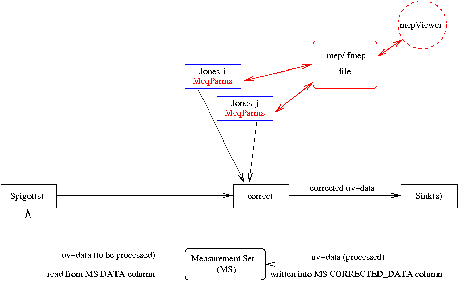
Figure 5 (click to enlarge)

Fig 5 shows how the uv-data may be corrected for instrumental errors. It is the inverse operation to the corruption of the nominal uv-data that we used before. The same Jones matrix subtrees are required, with the same MeqParm values in .mep or .fmep files. It is necessary to correct the uv-data from the MS to make a decent image.

However, it should be kept in mind that uv-data can only be corrected for a single point in the sky. Thus, in the presence of DDE's, it is imperative to subtract as many bright sources as possible from the uv-data, before transforming the residuals into an image. And even then, many separate "facet" images should be made, after correcting the uv-residials for the centre of the facet. The facet images should be small enough that the imaging errors to not increase "too much" towards the edge.

6. The Full Monty

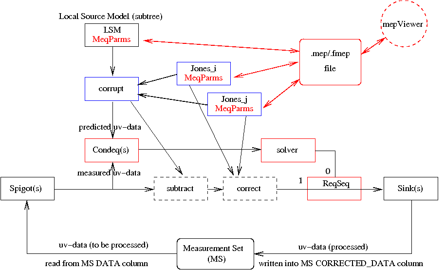
Figure 6 (click to enlarge)

Fig 6 is a combination of Figs 3,4,5. This is the prototype of a wide range of practical data reduction trees. First one solves for some subset of M.E. parameters. Then one uses the newly estimated MeqParm values to subtract the contributions of one or more LSM sources from the uv-data. And finally, the uv-residuals are corrected with the same MeqParm values.

Variations of this tree will be discussed in Nancay and beyond, in the context of 3GC. For instance, consider a cascade of such "peeling units", each of which "peels" a bright source from the uv-data, in reverse order of brightness.

Appendix: Some background information

Visibilities, uv-data and cohaerencies

The terms "uv-data" or "visibilities" or "cohaerency data" are all different names for the same thing, i.e. the output of a radio interferometry correlator. They are samples of the Fourier Transform of the observed brightness distribution. Thus, an image of the sky is obtained by Fourier Transforming the uv-data.

A radio aperture synthesis array consists of "stations" (a.k.a. "antennas" or "telescopes"). Each combination of two stations is called an "interferometer". An array of N stations has N(N-1)/2 different 2-station combinations.

Each station has two output signals, one for each polarization (X and Y for linear, or R and L for circular). The 2 output signals of each station are correlated with those of each of the other stations. The resulting visibilities for each combination (i,j) consist of 4 complex numbers, which are the elements of a 2x2 cohaerency matrix (e.g. XX XY YX YY). These are the uv-data units that are processed by MeqTrees.

The relative position of the stations (i and j) of an interferometer(i,j) is important. The (projected) distance and orientation of this "baseline", as seen from the observing direction, defines a point (u,v) in the so-called "uv-plane" (hence the name uv-data). An N-station array yields N(N-1)/2 different uv-samples simultaneously. Moreover, because of the rotation of the Earth, a slightly different set of uv-samples is obtained for each successive time interval, or "time-slot". An image of the sky is produced by Fourier-transforming the visibility function.

The resulting image will be convolved with a Point Spread Function (PSF), which is the Fourier Transform of the "uv-coverage", i.e. the sampling function of the uv-plane. Obviously, the PSF will have smaller sidelobes if the sampling of the uv-plane is more complete.

Since the PSF of a bright source will extend over the entire image, it will obscure fainter sources (which are often more interesting). Therefore, it is imperative to remove the PSF around bright sources. One way to do this is by means of image devonvolution methods like "CLEAN". But by far the best results are achieved by subtracting the bright sources from the uv-data, before turning them into an image.

The CASA / AIPS++ Measurement Set

The Measurement Set (MS) is organized as a table. The uv-data are stored in rows, in time order. Each table row contains a 4xNchan array of visibility data for all freq channels of a "spectral window", for all 4 correlations, of one particular interferometer (a pair of stations), for one "time-slot" (e.g. 1 minute).

MeqTrees also steps through the uv-data in time order. This is done by generating a series of processing Requests, each for a specified time-interval, which will be a multiple of the time-interval of a single MS row. The Requests are issued in parallel to the MeqSink nodes of the N(N-1)/2 subtrees of the available interferometers. These pass on the Request to their children, which pass them up the subtrees, right up to the MeqSpigot nodes that read uv-data from the DATA column of the MS. The processing Results are passed from node to node in the opposite direction, until the end Results are stored back in another column of the MS by the MeqSpigots.

The radio-astronomical Measurement Equation (M.E.)

Each Jones matrix may the product of other 2x2 Jones matrices, each of which represents a separate instrumental effect (e.g. phase).

To be continued.