SSSC1

This log goes through one of the scripts in the Calico framework designed for calibration of data from WSRT. It is divided into: 1. Examining the measurement set. 2. Making an image. 3. Source subtraction. 4. Doing some calibration.

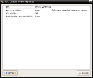
Opened the Cattery/Calico/calico-view-ms.py script, which is intended for any first-look at a Measurement Set. Compile time options were set up as in the screenshot - nothing else was done except pointing the script to the MS file before pressing 'Compile'.

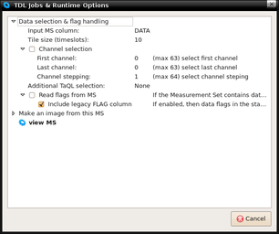
The runtime options window contains further options for data selection. The input MS column was set to 'DATA', since this is the only column filled for the simulated measurement sets.

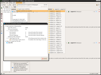
Opened bookmarks before clicking 'view MS' (see next entry).

From the SSSC page:

Before viewing the MS we can load a few bookmarks. These are pre-defined in the TDL script to allow visualisation of certain nodes in the tree.

With the runtime options window still open, these were selected from the bookmarks menu: Selected 'Inspect input visibilities' and one of the 'by baseline' options, before pressing 'view MS' in the TDL runtime options.

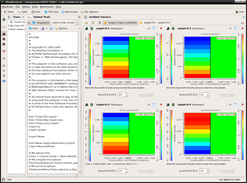
The screenshot shows amplitude (left) and phase (right) as a function of time (y-axis) and frequency (x-axis), with the colour scale indicating the value.

The phases are completely flat, consistent with a single point source at the phase centre. The variation in the amplitudes is due to the random antenna based gain errors we included.

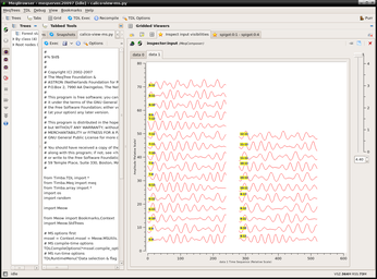
Pressing the 'inspect input visibilities' tab shows the amplitude versus time for each baseline (shown below in the 'inspector' screen shot).

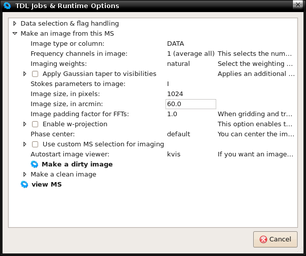
Selected the 'TDL Options' button to make an image from this MS. The imaging options were set up as shown in the screenshot before pressing 'Make a dirty image' -- this will then send the options to the lwimager (lightweight imager) from Casa-rest.

The image shows the central point source convolved with the PSF of the WSRT.

No automatic histograms were produced from my version of MeqTrees unfortunately (MeqTrees 1.0.1 [7207] on Ubuntu 9.04/64-bit).

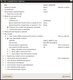
Restarted the MeqBrowser and loaded the Cattery/Calico/calico-wsrt.py TDL script. The compile time options window appeared and was set up as shown below.

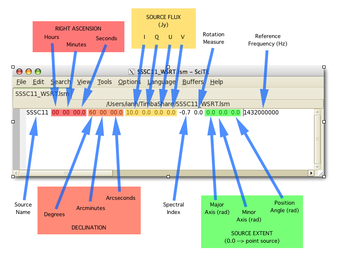
The sky model was downloaded from the SSSC page. Also included below is a very useful screenshot stolen from Ian Heywood which explains each column in the sky model file. For this measurement set, there is only one source, and the sky model is the same.

Pressed 'Compile' after setting all this up.

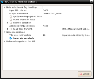
The runtime options were set up as below.

This adds spigots in the DATA column to read the data, subtracts the visibilities that correspond to the source model, and puts sinks in the CORRECTED_DATA column to write it.

Pressed 'Generate residuals'.

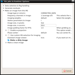
To image the residuals, I clicked the 'TDL Exec' button and expanded the 'Make an image from this MS' menu. Imaging needs to happen on the CORRECTED_DATA column, and the remaining options were set up as in the screenshot below.

Pressed 'Make a dirty image' - this resulted in the image as shown below.

When the simulation was generated, it included slowly varying receiver gain errors. The residual structure is a result of those errors. A sensible thing to do is try some calibration and solve for these errors in the G-jones matrix.

This section describes the first proper calibration step.

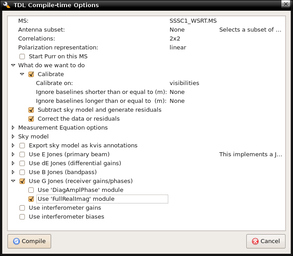
Selected the 'TDL Options' button to bring up the compile-time menu. Expanded the 'What we want to do' menu, checked 'Calibrate' and made sure calibration happens on the visibilities. Enabled 'subtract sky model' and 'correct the data or residuals'.

This time we're also solving for the values of a 2x2 gain matrix, the so-called G-Jones matrix. Selected the 'Use G-Jones (receiver gains/phases)' option, and checked the 'Use FullRealImag module' box. This solves for the real and imaginary parts of this matrix simultaneously.

Settings as in screenshot below -- then clicked 'Compile'.

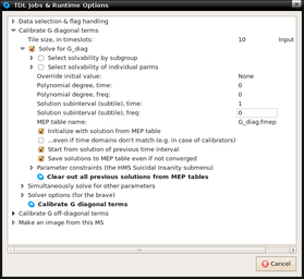
Run-time options appeared and were set up as in the screenshot. From Ian's page: The tile size is still set at ten, but we're also setting the solution sub-interval (sub-tile) for time to 1 and leaving frequency as 'none'. You can use this to set the number of solutions per tile, e.g. setting both to 1 would result in one solution per time and frequency point. We know that the gains are stable in frequency and variable with time, hence these values. One solution per time slot is more computationally expensive but it's also more accurate.

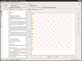
Opened 'Inspector G' bookmark and the residuals before pressing 'Calibrate G diagonal terms'.

Opened the 'TDL Exec' menu to image the new residuals. Expanded 'make an image from this MS' menu. Selected CORRECTED_DATA column, which should now contain residual visibilities (what's left after we've subtracted the source and corrupted the data with the G-Jones).

Selected 'Make a dirty image'. There is nano-Jy noise in the residual image. Presumably this is numerical noise, since there won't be real thermal noise from real receivers in this simulation.

This completes SSSC1.