SSSC6

Introduction from Ian's SSSC6 page: The WSRT records polarization in X and Y and produces four correlation products: XX XY YX YY.

For the simulations with unpolarized sources we've been assigning the source brightness solely to I and leave Q, U and V equal to zero.

The correlation products reflect this by having half the flux in XX, the other half in YY and nothing in the cross products.

For this first example we use a linearly polarized wave (i.e. V = 0), which is completely vertically polarized (i.e. psi = 0, Q = a positive value, U = 0).

The attached LSM in the data products below is the same as SSSC1 but with the Q value edited to be 10.0 Jy.

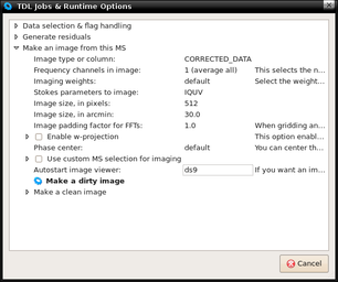
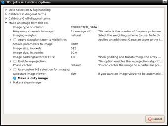
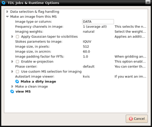
Using Cattery/Calico/calico-view-ms.py, pointing to the SSSC6 MS file. The imager run-time settings were set up to output all four Stokes parameters (I, Q, U and V) with options as shown. Pressed 'Make a dirty image'.

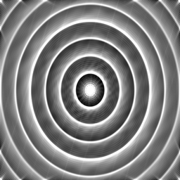
The source shows up in I and Q, not in U or V. (Had to use ds9 to view this file, as I couldn't figure out how to get Karma to display the other planes of the FITS cube).

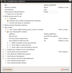
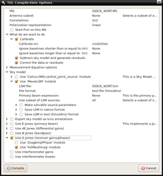
Using Cattery/Calico/calico-wsrt.py, with compile-time options as below, and using the supplied sky model.

Pressed 'Compile'.

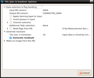
Runtime options set up as below (in run-time-1.png), before pressing 'Generate residuals'.

To image the residuals, selected 'TDL Exec' again with the options as below (in run-time-2.png).

Selected 'TDL Options' and set things up as in the screenshot below.

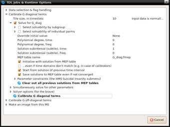
Pressed 'Compile' and set the run-time options up as below, before pressing 'Calibrate G diagonal terms'.

To image the new residuals, opened 'TDL Exec' button. Expanded 'make an image from this MS' menu. Selected CORRECTED_DATA column, then 'Make a dirty image'. (Set up as in calico-wsrt-imaging-options-residuals.png).