SSSC6 PURR Logs

SSSC6 PURR Logs


Contact Details

Logged on 19/08/09 11:26:57

Stewart Gleadow, gleadows@unimelb.edu.au, University of Melbourne


Sanity Check MS

Logged on 19/08/09 11:34:18

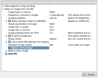
Using calico-view-ms.py

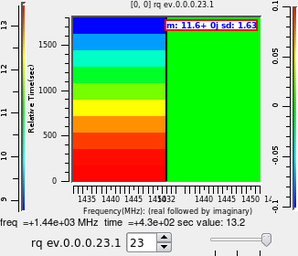
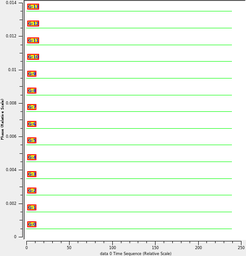
View visibility data for some baselines, just to to a quick sanity check on the MS, see that it contains data that resembles that expected.

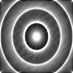
Create a dirty image of the uncalibrated data, check that it looks like there is a source convolved with the PSF of WSRT in the centre of the beam in Stokes I and Q, but not in U and V.

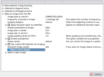
Averaging all freq channels into one to keep file sizes small.

Data products

image_dirty_runtime.png

image_dirty_runtime.png

SSSC6_WSRT.MS.DATA.channel.1ch.fits (header)

1x4x512x512 FITS cube, 4 planes are given below.

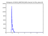
0-full.png0-hist-full.png
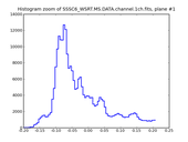
0-hist-zoom.png

Image plane #0.

data range:-0.198724,4.98532
mean:-0.00616115
sigma:0.122663
clipping:95%
clip range:-0.198724,0.211342
1-full.png1-hist-full.png
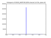
1-hist-zoom.png

Image plane #1.

data range:-0.198724,4.98532
mean:-0.00616115
sigma:0.122663
clipping:95%
clip range:-0.198724,0.211342
2-full.png2-hist-full.png
2-hist-zoom.png

Image plane #2.

data range:0,0
mean:0
sigma:0
clipping:95%
clip range:0,0.000976562
3-full.png3-hist-full.png
3-hist-zoom.png

Image plane #3.

data range:0,0
mean:0
sigma:0
clipping:95%
clip range:0,0.000976562
some_visibility_data.png

some_visibility_data.png


Gain Calibration

Logged on 19/08/09 11:48:48

Using calico-wsrt.py

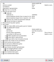
Set compile options to calibrate G-Jones on visibilities, and subtract LSM, shown in image below.

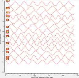
Pre-load the bookmark for inspector:G, so that we can see the gain solutions. Expect them to be varying perioically in amplitude but flat in phase, as shown below.

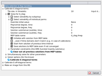
Run the script to calibrate G diagonal terms, shown in image below.

Data products

gain_solution_phase.png

gain_solution_phase.png

gain_solution_amplitude.png

gain_solution_amplitude.png

gain_cal_runtime.png

gain_cal_runtime.png

gain_cal_compile.png

gain_cal_compile.png


Image Residuals

Logged on 19/08/09 11:55:25

Now that we have calibrated the gains, image the residuals from LSM (again using calico-wsrt.py).

Average all frequency channels together, since we know the gain solution is the same for all channels, and to keep file size down (see runtime settings below).

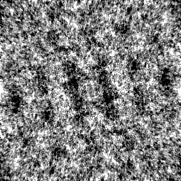
Expect to see nano Jy level noise remaing in Stokes I and Q, indicating that the model has been accurately removed and the calibration successful, and nothing in Stokes U and V as there was never any signal in those channels, and we have not included any instrumental leakage.

Data products

image_residuals.png

image_residuals.png

SSSC6_WSRT.MS.CORRECTED_DATA.channel.1ch.fits (header)

1x4x512x512 FITS cube, 4 planes are given below.

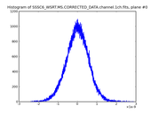
0-full.png0-hist-full.png
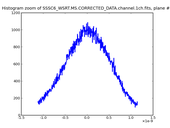
0-hist-zoom.png

Image plane #0.

data range:-2.39581e-09,2.90325e-09
mean:4.52573e-12
sigma:5.71659e-10
clipping:95%
clip range:-1.1228e-09,1.14897e-09
1-full.png1-hist-full.png
1-hist-zoom.png

Image plane #1.

data range:-2.39581e-09,2.90325e-09
mean:4.52573e-12
sigma:5.71659e-10
clipping:95%
clip range:-1.1228e-09,1.14897e-09
2-full.png2-hist-full.png
2-hist-zoom.png

Image plane #2.

data range:0,0
mean:0
sigma:0
clipping:95%
clip range:0,0.000976562
3-full.png3-hist-full.png
3-hist-zoom.png

Image plane #3.

data range:0,0
mean:0
sigma:0
clipping:95%
clip range:0,0.000976562

.tdl.conf


This log was generated by PURR version 1.0.