
The following software is freely available. However, if you use it for published research, you are requested to cite the paper where the method is described, highlighted in red. You are not allowed to re-distribute any of these programs (modified or not) without explicit permission from the author.
NOTE: an outdated version of my programs in the ![]() language is also available HERE, however I strongly recommend the Python version.
language is also available HERE, however I strongly recommend the Python version.
My packages above are on the Python Package Index (PyPI).
See my review on galaxy structure and evolution: ![]()
|
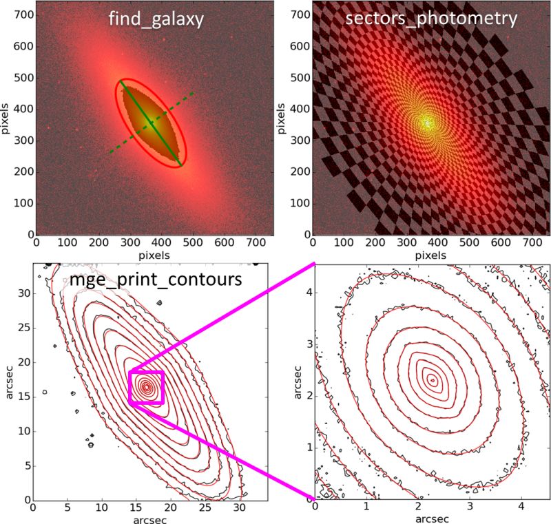
Illustration of the steps involved in the MGE fit to the S0 galaxy NGC 4342 using the MgeFit package. The figures were produced by the mge_fit_example.py script included in the Python distribution of the software.
|
This software obtains an accurate Multi-Gaussian Expansion (MGE) parameterizations (Emsellem et al. 1994; Cappellari 2002) for a galaxy surface brightness with the fitting algorithm of Cappellari (2002, MNRAS, 333, 400). Given that Gaussians are not orthogonal functions, MGE fits are in general strongly degenerate, with difficult global convergence, but the MGE_FIT_SECTORS method solves all problems, making MGE fitting an automated, reliable and robust process.
See Cappellari et al. (2013) for a large scale application of this software to the study of the M/L ratio and the Fundamental Plane of early-type galaxies and Cappellari et al. (2012, Nature) for an application to the study of the stellar IMF. The MGE parameterization is useful in the construction of realistic dynamical models of galaxies (see JAM modelling below), for PSF deconvolution of images, for the correction and estimation of dust absorption effects, or for galaxy photometry.
MgeFit package in The source code of the MgeFit package, including four test galaxy images, is on the Python Package Index (PyPI). It was last updated on the 31 March 2023 and the changes are documented in the CHANGELOG.
How to install: Use "pip install mgefit". Without write access to the global site-packages directory, use "pip install --user mgefit".
Usage examples: are in the directory "examples" inside the main package folder inside site-packages.
MgeFit requires the scientific core packages NumPy, SciPy and Matplotlib, and the examples use Astropy to read FITS images (it was tested with Python 3.10 using Numpy 1.22, SciPy 1.8 and Matplotlib 3.5).
Also included in the MgeFit package is the mpfit implementation by Markwardt (2009) of the MINPACK (Moré, Garbow & Hillstrom, 1980) Levenberg-Marquardt nonlinear least-squares optimization algorithm. The mpfit routine was translated into Python by Mark River and updated here for NumPy by Sergey Koposov. I modified the latter version to support Python 3 and fixed some numerical instabilities. Note that MgeFit uses the mpfit implementation instead of the SciPy.optimize.least_squares one, because of the ability of mpfit to tie parameters or keep them fixed.
NOTE: I would appreciate if you drop me an e-mail (address at the bottom) when you download the above procedures.
|
|
2. Jeans Anisotropic MGE (JAM) Modelling |
| Jeans Anisotropic MGE modelling of the dynamics, stellar kinematics or proper motions of axisymmetric or spherical galaxies |
|
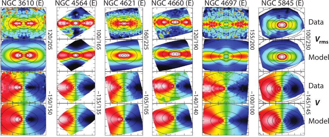
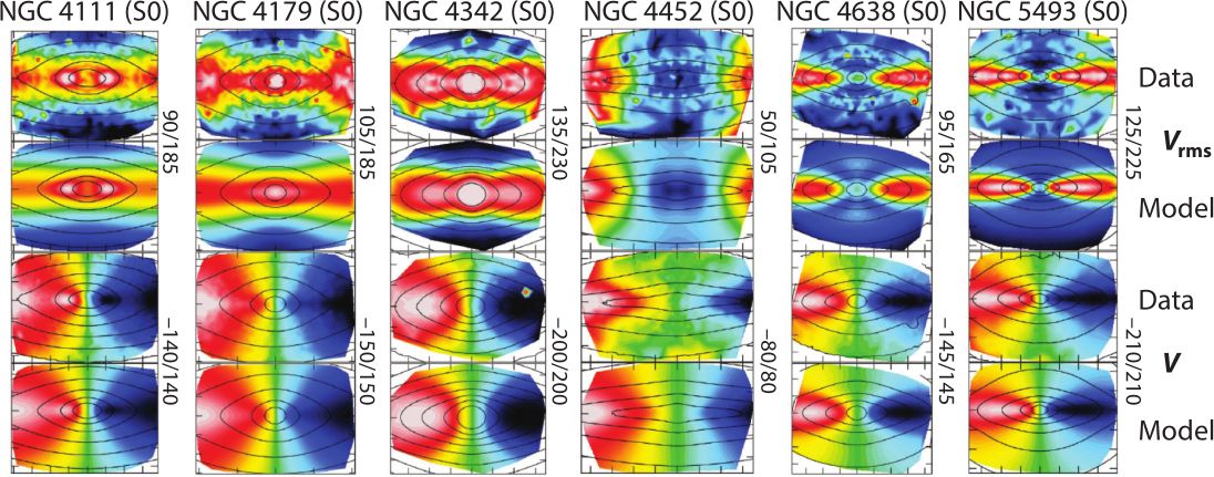
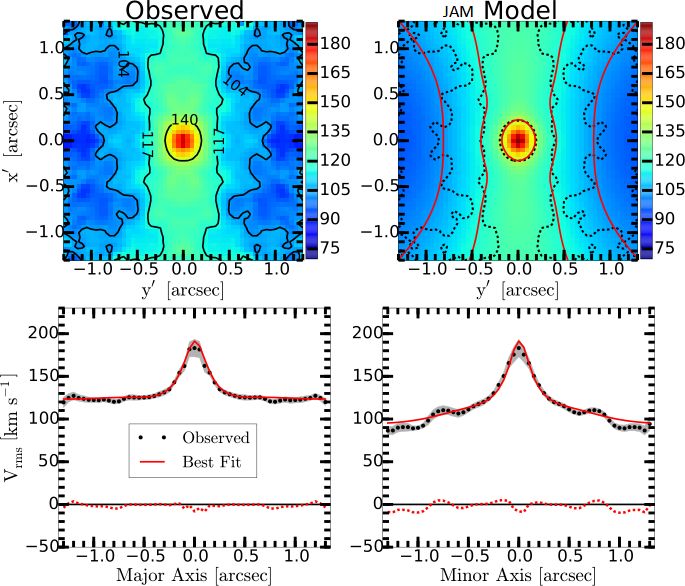
| Figure 1: Examples of JAM data-model comparisons. The bi-symmetrized SAURON stellar kinematics of 6 Elliptical (left) and 6 S0 (right) fast-rotator early-type galaxies is compared to the predictions of the anisotropic Jeans models with JAM. The kinematics varies widely for different galaxies, yet these two-parameters (!) models are able to correctly predict the shape of a pair of two-dimensional functions (V and Vrms), once the observed surface brightness is given (this is fig.10 of Cappellari 2016, ARA&A). |
|
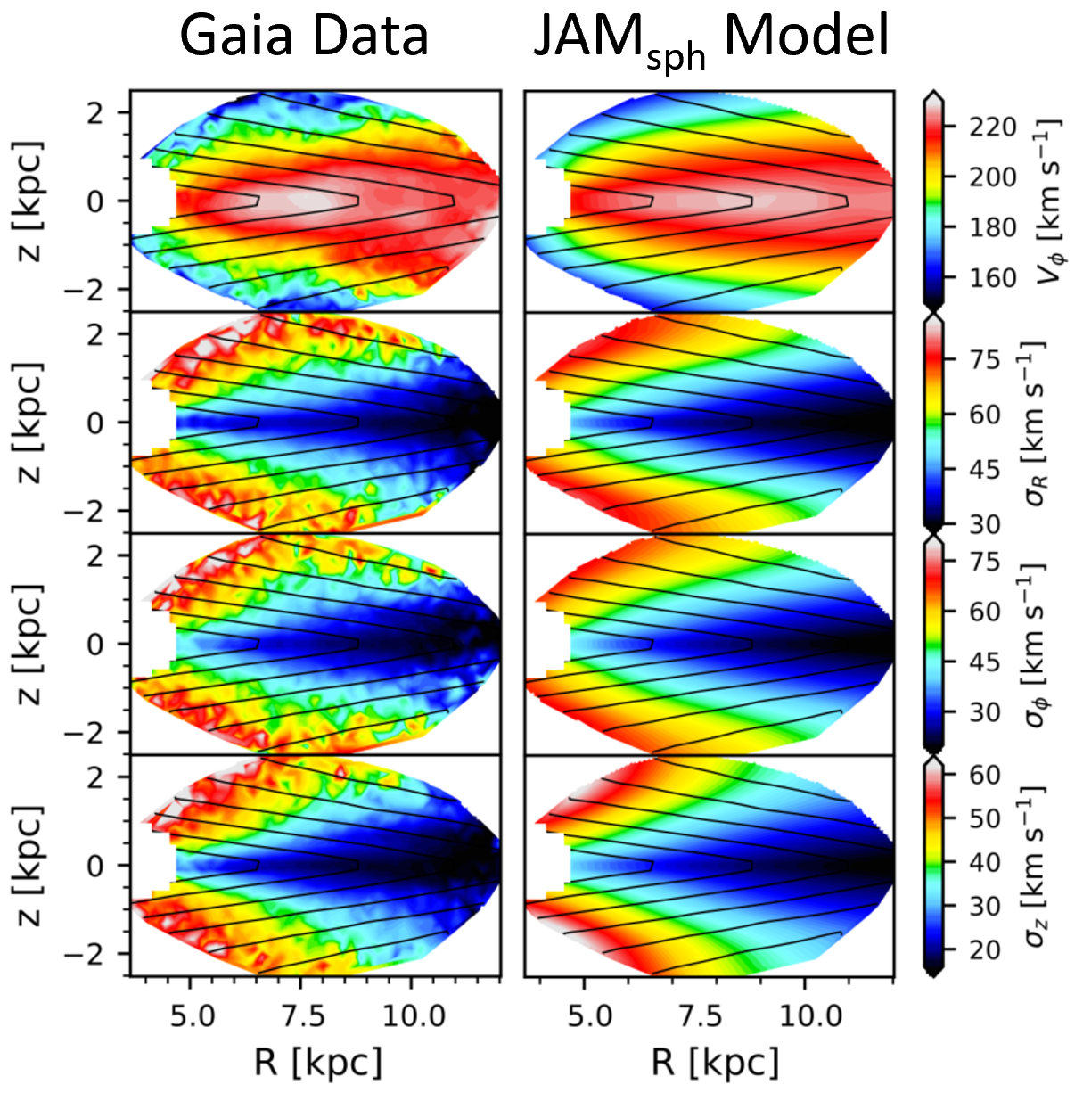
| Figure 5: This is the first dynamical modelling (using JAMsph) of the high-quality Gaia DR2 kinematics of the Milky Way, with full 6D phase-space coordinates. For the first time, there are no dynamical degeneracies and the model has no freedom to fit the data, yet all features are reproduced. This is an important test of galaxy dynamics. (figure taken from Nitschai et al. 2020) |
|
| Figure 4: Validating black hole (BH) recovery with JAM. A detailed JAM modelling accurately recovers the "benchmark" BH mass in NGC4258, as inferred from maser observations (figure taken from Drehmer et al. 2015). An equally good agreement was found with JAM for the "benchmark" BH in the Milky Way (Sec.4.1.2 of Feldmeier-Krause et al. 2017). Other successful BH comparisons, between JAM and Schwarzschild's method, were presented e.g. in Cappellari et al. (2010), for 25 galaxies, and Krajnović et al. (2018), for 7 galaxies. |
|
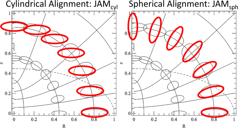
| Figure 3: The JAM package includes an implementation for both the cylindrically-aligned solution JAMcyl of Cappellari (2008) and the spherically-aligned solution JAMsph of Cappellari (2020). Comparisons between these two extreme solutions allows for a robust assessment of possible systematic modeling uncertainties (see Cappellari 2020 for some examples). |
|
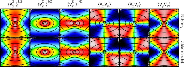
| Figure 2: Including both proper motions and radial velocities. Top Panels: the components of the symmetric velocity second moment tensor measured from the particles of a realistic N-body simulation. Bottom Panels: the corresponding JAM model predictions. Note the striking agreement! (Cappellari 2012) |
The JAM software in this section can be used for the dynamical modelling of galaxies or other gravitationally-bound systems of particles. It was used e.g. to measure the mass of supermassive black holes in galaxies, to infer their dark-matter content or to measure galaxy masses and density profiles.
JAM implements a solution of the Jeans equations which allows for orbital anisotropy (three-integrals distribution function) and also provides the full second moment tensor, including both proper motions and radial velocities, for both axisymmetric (Cappellari 2012) and spherical geometry (Cappellari 2015). The technique was introduced in Cappellari (2008), for the cylindrically-aligned case, and in Cappellari (2020), for the spherically-aligned case (Figure 3), and I called it the Jeans Anisotropic Modelling (JAM) method. It relies on the Multi-Gaussian Expansion parameterization (Emsellem et al. 1994; Cappellari 2002) for the galaxy surface brightness.
With the addition of a single extra parameter βz=1-(σz/σR)2 (in cylindrical alignment) or β=1-(σθ/σr)2 (in spherical alignment), the simple and user-friendly three-integrals JAM method already provides a dramatic improvement over the classic but less general two-integrals f(E,Lz) Jeans (1922) models. However JAM also allows for tangential anisotropy γ=1-(σφ/σR)2 and/or for spatially varying anisotropy (different for every MGE Gaussian). The JAM models provide a remarkably good descriptions of state-of-the-art integral-field stellar kinematics of real galaxies (Figure 1). This makes the technique well suited to measure the inclination, the dynamical M/L and angular momenta of early-type fast-rotators and spiral galaxies.
The JAM routines are designed for axisymmetric or spherical geometry, (i) they can provide the proper motion dispersion tensor (Cappellari 2012; Cappellari 2015; Figure 2), (ii) allow for the inclusion of dark matter, (iii) variable stellar M/L, (iv) spatially varying anisotropy and (v) multiple kinematic components and (vi) supermassive black holes (BH; Figure 4). The JAM package also includes a routine to compute the circular velocity from the MGE models. Some sample applications of the JAM method are given below:
To construct dynamical models with the JAM method one needs to describe the galaxies surface brightness via the Multi-Gaussian Expansion parametrization using my MGE_FIT_SECTORS package above.
|
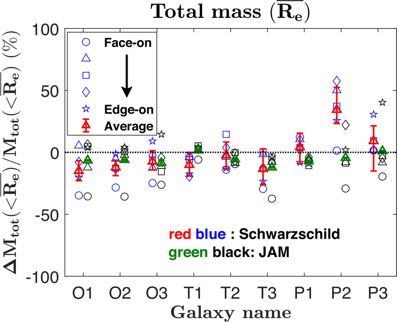
| Figure 7: JAM works better than Schwarzschild on simulated galaxies. A detailed comparison using the Illustris simulations with the JAM and Schwarzschild's (SCH) dynamical models, found that JAM recovers the known enclosed total mass within 1Re more accurately than SCH. Specifically, the 68th percentile deviation (1σ error) over all 45 model fits is 1.6× smaller for JAM than SCH (This is Fig.4 from Jin et al. 2019). |
|
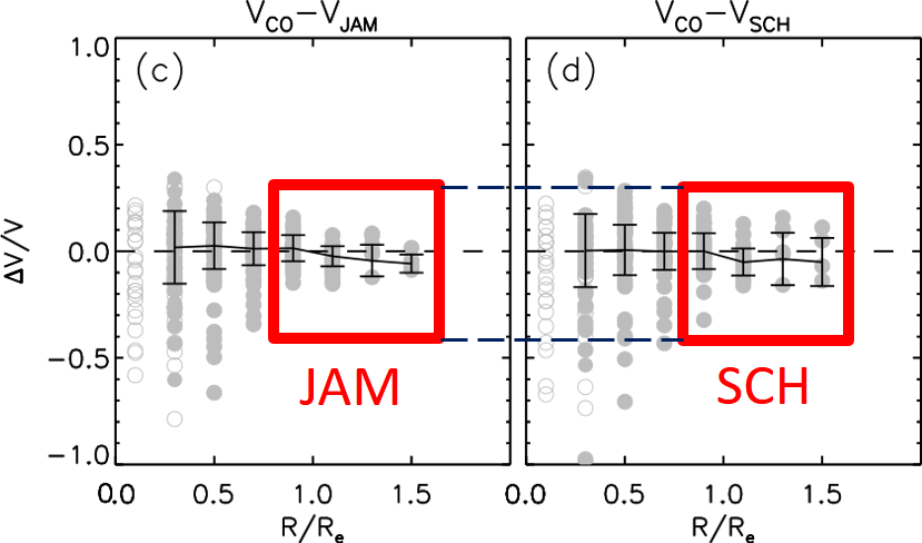
| Figure 6: JAM works better than Schwarzschild on real galaxies. A detailed comparison, for 54 real disk galaxies with CALIFA data, between the circular velocity VCO measured from CO gas and the corresponding VJAM and VSCH from dynamical modelling of integral-field stellar kinematics using the JAM and Schwarzschild's (SCH) methods, found that JAM recovers the densities more accurately than SCH. Specifically, between 0.8-1.6 Re (inside the red boxes), where the gas is well-resolved and Vc is better determined, the mean 1σ error is 1.7× smaller for JAM than SCH (This is Fig.8 from Leung et al. 2018). |
The source code of the JamPy package is on the Python Package Index (PyPI). It was last updated on the 21 July 2023 and the changes are documented in the CHANGELOG.
How to install: Use "pip install jampy". Without write access to the global site-packages directory, use "pip install --user jampy".
Usage examples: are in the directory "examples" inside the main package folder in site-packages.
Also required is my plotbin package (automatically installed by pip).
The JamPy package requires the scientific core packages NumPy, SciPy and Matplotlib (it was tested with Python 3.11 using Numpy 1.24, SciPy 1.9 and Matplotlib 3.6).
NOTE: I would appreciate if you drop me an e-mail (address at the bottom) when you download the above procedures.
|
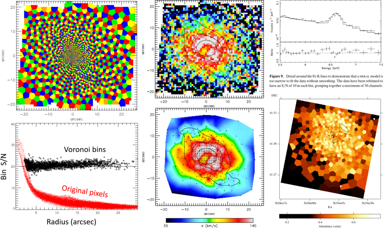
| Left: Four-coloring of Voronoi binning; Middle: Unbinned versus Voronoi binned stellar kinematics from Integral-Field Spectroscopy (Cappellari & Copin 2003); Right: Voronoi binning of abundance from X-ray data (Sanders et al. 2004). |
|
|
3. The Voronoi binning method (VorBin) |
| Adaptively spatial bin two-dimensional data to a constant signal-to-noise ratio per bin |
The Voronoi Binning method of Cappellari & Copin (2003, MNRAS, 342, 345) optimally solves the problem of preserving the maximum spatial resolution of general two-dimensional data (or higher dimensions), given a constraint on the minimum signal-to-noise ratio.
The Voronoi binning method has been applied to a variety of types of data. A review of the concepts and applications to (i) X-ray data, (ii) integral-field spectroscopy, (iii) Fabry-Perot interferometry, (iv) N-body simulations, (v) standard images and (vi) other regularly or irregularly sampled data is given in Cappellari (2009).
The source code of the VorBin package, with examples and instructions, is on the Python Package Index (PyPI). It was last updated on the 24 February 2022 and the changes are documented in the CHANGELOG.
How to install: Use "pip install vorbin". Without write access to the global site-packages directory, use "pip install --user vorbin".
User Manual: Is available on THIS PAGE (most up-to-date) or as PDF.
Usage example: is in the package folder inside site-packages.
The VorBin package requires the scientific core packages NumPy, SciPy and Matplotlib (it was tested with Python 3.10 using Numpy 1.22, SciPy 1.8 and Matplotlib 3.5).
My optional plotbin package contains routines to visualize Voronoi 2D-binned or unbinned data like in the figures above.
NOTE: I would appreciate if you drop me an e-mail (address at the bottom) when you download the above procedures.
|
|
4. Penalized PiXel-Fitting (pPXF) |
| Stellar or gas kinematics and stellar population from galaxy spectra via full spectrum fitting with photometry |
|
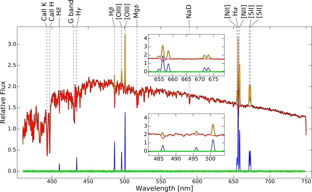
| Figure 1: Stellar and gas kinematics fit with pPXF. The black line (mostly hidden by the fit) is the relative flux of the observed spectrum. The red line is the pPXF fit for the stellar component, while the orange line is a fit to the gas emission lines. The green symbols at the bottom are the fit residuals, while the blue lines is the gas-only best-fitting spectrum. The main absorption and emission features are indicated at the top of the plot (taken from Cappellari 2017). |
This software implements the Penalized PiXel-Fitting method (pPXF) to extract the stellar or gas kinematics and stellar population from absorption-line spectra of galaxies, using a maximum penalized likelihood approach. The method was originally described in Cappellari & Emsellem (2004) and was significantly upgraded in subsequent years and particularly in Cappellari (2017) and with the inclusion of photometry and linear constraints in Cappellari (2023). The method is very general and robust. For this reason it was applied to a variety of situations. The following key features are implemented in the current pPXF program:
See Emsellem et al. (2004, SAURON), Cappellari et al. (2011, ATLAS3D), Falcon-Barroso et al. (2017, CALIFA), van de Sande et al. (2017, SAMI) and Westfall et al. (2019, MaNGA) for some ever increasing large-scale applications of the pPXF method to the measurement of the stellar or gas kinematics of galaxies. Cappellari et al. (2009) demonstrates the use of pPXF to measure the stellar velocity dispersion of a sample of passive galaxies at redshift z~2.
The ability of the pPXF method to fit a large set of stellar templates together with the kinematics allows the template mismatch problem to be virtually eliminated. This is particularly useful given the current availability of large stellar libraries spanning wide ranges of physical parameters and having good spectral resolution. Excellent results have been obtained by using a few hundred template stars with pPXF, from which generally about 10-20 are selected by the program to provide detailed fits to high S/N galaxy spectra. An extensive account of the available stellar libraries is maintained by David Montes. An incomplete list of libraries that have been successfully used with pPXF for the kinematics extraction is given below:
|
|
|
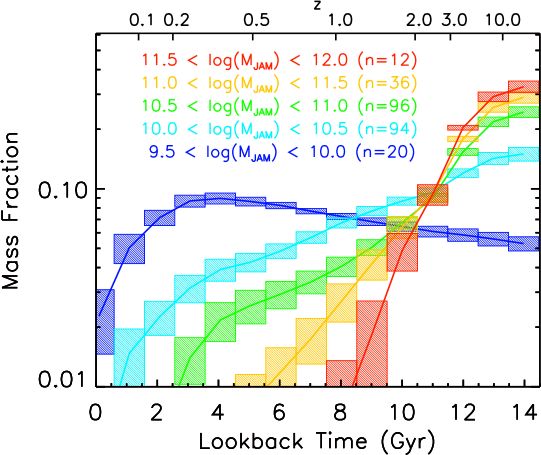
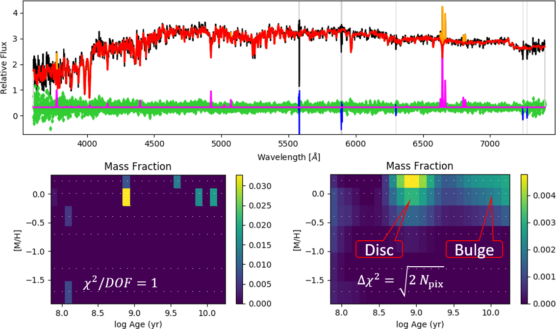
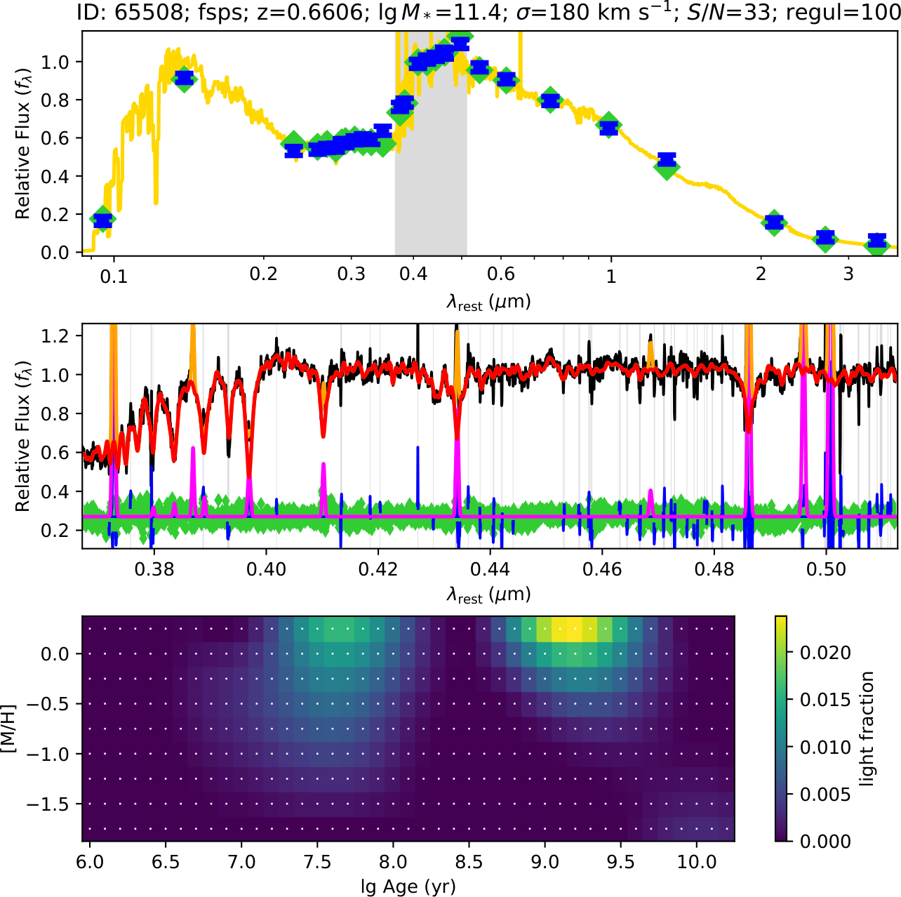
| Figure 2: Star-formation history with pPXF. The plot shows the star-formation history of ATLAS3D galaxies, in bins of different galaxy stellar mass. This was recovered with pPXF using regularization (taken from McDermid et al. 2015). | Figure 3: Population and gas with pPXF. The plots show the pPXF fit to a MaNGA spectra for the spiral galaxy NGC2916 (from SDSS DR13). The "Mass Fraction" map show the pPXF solution in different age and metallicity intervals. The Left Map has no regularization and is noisy as the population inverse problem is ill-posed. Regularization is a standard approach to solve ill-posed problems (see Cappellari 2017, Sec.3.5). The Right Map show the regularized solution. The fit used 24(Ages)×6([M/H])=144 MILES population templates by Vazdekis et al. (2010), and 12 gas emission lines. | Figure 4: Spectra and photometry with pPXF. The top panel show a fit to the 28-bands COSMOS photometry for a galaxy in the LEGA-C survey at redshift z∼0.7. The grey band indicates where the spectrum is also available. The middle panel is the fit to the spectrum and gas emission. The bottom panel shows the recovered star formation history (SFH) using 43(Ages)×9([M/H])=387 FSPS population templates (taken from Cappellari 2022). |
pPXF is the most efficient, reliable and flexible public implementation of the so called "Full-Spectrum Fitting" method to study stellar populations. This technique has replaced the traditional use of line-strength indices, due to the availability of high-quality model spectra. pPXF was designed to be independent on any specific set of stellar-population models and has already been used with nearly every available one. An usage example, using the Vazdekis's models, is included with permission in the pPXF package. This can be easily adapted by users to employ pPXF with other stellar-population models. An incomplete list of the main stellar population models that were used with pPXF is the following:
pPXF allows one to extract multiple kinematic components, with different stellar populations, from a spectrum. Gas emission lines can be fitted simultaneously, avoiding the need for masking them. This is particularly useful when studying the stellar population of galaxies with prominent emission lines (e.g. the Balmer lines) filling important absorption features (see Figures 1 and 3).
Please also cite the source of the E-MILES stellar population models (Vazdekis et al. 2016) if you use pPXF with the included library of spectral templates.
A number of similar, but less optimized and less general implementations of the Full Spectrum Fitting method exist (e.g. STARLIGHT by Cid Fernandes et al. 2005; STECMAP by Ocvirk, et al. 2006; VESPA by Tojeiro et al. 2007). A major limitation of most available codes is that they ignore the fact that the recovery of the star formation history and chemical composition distribution from the galaxy spectra is an ill-posed problem. A standard technique to solve ill-posed problems is regularization (see Cappellari 2017, Sec.3.5), which is invoked in pPXF via the keyword REGUL. Regularization is essential to make sense of the derived star formation histories and to explore model degeneracies (see Figure 2 and 3). The regularized solution has a simple Bayesian interpretation: it represents the most likely solution for the weights, given an adjustable prior on the amplitude of the fluctuations.
See Cappellari et al. (2012, Nature) for an early pPXF study of the M/L and IMF of stellar populations.
The source code of the ppxf package, with examples and instructions, is on the Python Package Index (PyPI). It was last updated on the 6 July 2023 and the changes are documented in the CHANGELOG.
How to install: Use "pip install ppxf". Without write access to the global site-packages directory, use "pip install --user ppxf".
User Manual: Detailed documentation is on THIS PAGE (always up to date) or from here as PDF ppxf_manual.pdf.
Usage examples: ![]() Notebooks
Notebooks ppxf examples are available HERE. Python examples are in the directory "examples" inside the main ppxf package folder inside site-packages.
ppxf requires the scientific core packages NumPy, SciPy and Matplotlib, and the examples use Astropy to read FITS data (it was tested with Python 3.10 using Numpy 1.22, SciPy 1.8 and Matplotlib 3.5).
NOTE: I would appreciate if you drop me an e-mail (address at the bottom) when you download the above procedures.
|
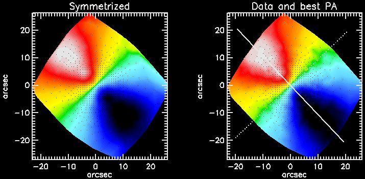
| Best fitting symmetrized kinematics of NGC 2974 |
This software implements the method presented in Appendix C of Krajnovic et al. (2006, MNRAS, 366, 787) to measure the global kinematic position-angle (PA) from integral field observations of a galaxy stellar or gas kinematics.
See Cappellari et al. (2007) and Krajnovic et al. (2011) for two large scale application of this software to the study of the stellar kinematical misalignment of early-type galaxies. See Davor's Krajnovic page for the related Kinemetry package.
PaFit package in The PaFit package is on the Python Package Index (PyPI). It was last updated on the 3 April 2023.
How to install: Use "pip install pafit". Without write access to the global site-packages directory, use "pip install --user pafit".
Also required is my plotbin package (automatically installed by pip).
PaFit requires the scientific core packages NumPy and Matplotlib (it was tested with Python 3.10 using Numpy 1.22 and Matplotlib 3.5).
NOTE: I would appreciate if you drop me an e-mail (address at the bottom) when you download FIT_KINEMATIC_PA.
|
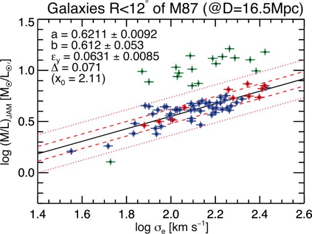
Figure 1: Fitting of the (M/L)-σ relation in the Virgo cluster using LTS_LINEFIT (taken from Cappellari et al. 2013a). The green outliers above the relation are automatically removed from the fit. They turn out to be background galaxies and for this reason they do not follow the cluster relation.
|
This software implements the method presented in Sec. 3.2 of Cappellari et al. (2013a, MNRAS, 432, 1709) to to perform extremely robust fit of lines or planes to data with errors in all variables, possible large outliers (bada data) and unknown intrinsic scatter.
The code combines the Least Trimmed Squares (LTS) robust technique, proposed by Rousseeuw (1984) and speeded up in Rousseeuw & Van Driessen (2006), into a least-squares fitting algorithm which allows for intrinsic scatter and errors in all coordinates. This method makes the fit converge to the correct solution even in the presence of a large number of catastrophic outliers (like in Figure 1), where the much simpler σ-clipping approach can converge to the wrong solution.
LtsFit package in The LtsFit package is on the Python Package Index (PyPI). It was last updated on the 20 July 2023.
How to install: Use "pip install ltsfit". Without write access to the global site-packages directory, use "pip install --user ltsfit".
Usage examples: are in the directory "examples" inside the main package folder inside site-packages.
LtsFit requires the scientific core packages NumPy, SciPy and Matplotlib (it was tested with Python 3.10 using Numpy 1.22, SciPy 1.8 and Matplotlib 3.5).
NOTE: I would appreciate if you drop me an e-mail (address at the bottom) when you download LTS_LINEFIT and LTS_PLANEFIT.
|
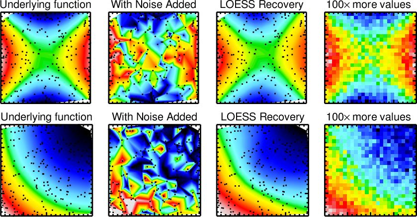
Application of the CAP_LOESS_2D routine (with FRAC=0.6) to the recovery of two underlying functions from a noisy distribution of 200 scattered values. For comparison, the right panels show the distribution obtained via simple averaging on a grid, but using 100× more values than the ones used for the LOESS recovery. The LOESS approach achieves a comparable result while requiring a much smaller number of input values.
|
This software provides an improved implementation of the one-dimensional (Cleveland 1979) and two-dimensional (Cleveland & Devlin 1988) Locally Weighted Regression (LOESS) method to recover the mean trends of the population from noisy data in one or two dimensions. It includes a robust approach to deal with outliers (bad data).
These programs were implemented and used to produce the two-dimensional maps and the one-dimensional mean trends in Cappellari et al. (2013b, MNRAS, 432, 1862).
loess package in The loess package is on the Python Package Index (PyPI). It was last updated on the 31 Jan 2022 (it was tested with Python 3.10 using Numpy 1.22 and Matplotlib 3.5).
How to install: Use "pip install loess". Without write access to the global site-packages directory, use "pip install --user loess".
Usage examples: are in the directory "examples" inside the main package folder inside site-packages.
Also required to run the 2D example is my plotbin package (automatically installed by pip).
NOTE: I would appreciate if you drop me an e-mail (address at the bottom) when you download the code.
|
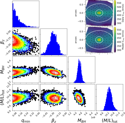
Figure 1: Corner plot for the posterior of the model parameters obtained when fitting the black hole mass in the galaxy NGC1277 using the jam modelling method and the AdaMet Bayesian code (taken from Krajnovic et al. 2018). The Python code to produce this figure is included in the JamPy package above.
|
This AdaMet package is the implementation of Cappellari et al. (2013a, MNRAS, 432, 1709) of the Adaptive Metropolis algorithm of Haario (2001). In many real-world applications, it was found to be more efficient and robust than the emcee approach, whose warm-up phase scales linearly with the number of walkers. For this reason, and because of its didactic value, the AdaMet code is provided here as an alternative.
AdaMet package in The user-friendly AdaMet package is on the Python Package Index (PyPI). It was last updated on the 6 October 2020 (it was tested with Python 3.10 using Numpy 1.22 and Matplotlib 3.5).
How to install: Use "pip install adamet". Without write access to the global site-packages directory, use "pip install --user adamet".
Usage examples: are in the directory "examples" inside the main package folder inside site-packages.
Also required for plotting is my plotbin package (automatically installed by pip).
Comments and suggestions are welcome to the address michele.cappellari@physics.ox.ac.uk
Latest changes: 4/Sep/2023
Go back to Michele Cappellari Homepage