Before we proceed, let's repeat the corrupted simulation above, but this time write the results to the DATA column. When you get genuine radio telescope data from an observatory this is where your raw visibility measurements live. If you haven't changed anything from the last run, then just click TDL Exec, change the 'Output MS column' to 'custom', enter 'DATA' in the relevant box and re-simulate the visibilities.

Once this is done, let's use a calibration script to try to get rid of the corruptions we've just put in. As well as the 'Siamese' simulation framework, there are some example calibration scripts in the Cattery under the 'Calico' folder.

Close and restart the meqbrowser, select 'Load TDL script' from the TDL menu, and open calico-wsrt-tens.py. As with the simulation script, this takes a Measurement Set and a sky model and constructs a measurement equation with various image plane and uv-plane terms in it. The difference here is that the Measurement Equation contains solvable parameters, and instead of simply predicting data and writing it to the MS, it predicts data and compares this to the existing data the that MS contains. A numerical solver minimises the difference between the observed and the predicted by tuning the solvable parameters.

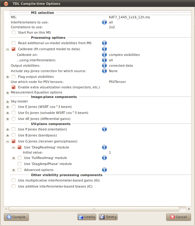
The Measurement Equation paradigm offers ridiculous amounts of flexibility, as partially evidenced by the daunting amount of compile time options in that popped up when the script laoded, but all we'll be solving for here are the G-Jones terms, i.e. a single solvable complex gain term for each element of the array. Most of the options can be ignored for now.

Point the script at the Measurement Set that contains the simulated visibilities, and as before in the skymodel section select the "Use 'TiggerSkyModel' module" and load sumss_dec-74_field.lsm.html. Our assumed sky model here is the central point source only, i.e. source 43_J1930M76.

So far, so simulation.

The first new part here is the 'Processing options' section. Check 'Calibrate (fit corrupted model to data)', we want to 'Calibrate on:' 'complex visibilities', and set the 'Output visibilities:' to 'corrected data'. Check also 'Enable extra visualization nodes (inspectors etc.)' as bookmarks are always useful and we'll want some in a minute.

As mentioned above we're just solving for the G-Jones terms here, so check 'Use G Jones (receiver gains/phases)' ad select "Use 'DiagRealImag' module". This just sets up a 2x2 Jones matrix for each antenna with solvable terms on the diagonal (XX/YY).

Click 'Compile' and the meqbrowser will build your calibration tree.

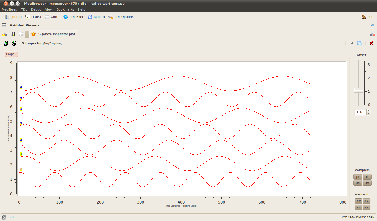
The runtime options should pop up now, but before we look at those let's open a bookmark. If you only open one bookmark this session let's make it the 'G Jones: inspector plot' one.

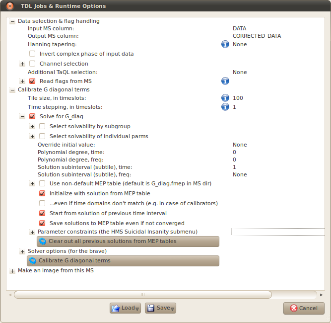
There are a few more options in the run time menu than we are used to with the simulation script. An important pair to get right is the 'Input MS column' and 'Output MS column' in the 'Data selection & flag handling' menu. Expand this and check that the former says DATA and the latter CORRECTED_DATA. This ensures we're solving for the gain terms in our parametrized Measurement Equation by comparing them to the correct 'observations', i.e. the results of our corrupted simulation. The observed DATA will be divided by the best fitting gain terms at the end of the calibration, and the resulting visibilities written to CORRECTED_DATA for imaging or further processing. The calibration process is (and should be) non-destructive, preserving our original measurements at all times. (That doesn't mean you don't need a backup, though!)

The other thing I've checked here is the 'Read flags from MS' option. In a real observation you don't want to be solving for data that you've flagged as RFI for example. When I made this simulated KAT-7 MS I included flagging for antenna elevations below a certain threshold, although to be honest I'm not sure this threshold is ever reached at this Declination. I suppose I should look at the flag columns in the MS...

Moving onwards: expand the 'Calibrate G diagonal terms' submenu. Most of these values can be left at their defaults. The important one is the 'Tile size, in timeslots'. The timeslot in this case is whatever the native time resolution of the MS is (I believe it's 30 seconds, but you can collect bonus points by having a look at the EXPOSURE column in the main table if you're curious). Anyway, what setting this parameter does is determine how much of the data MeqTrees reads in at a time. For a job of this size on a decent spec machine you can probably set this pretty high. I've set it to 100 here. The G Jones option in this calibration script by default reads in all frequency channels, but our simulation only has one so this is not an issue. The 'Time stepping, in timeslots' option remains at 1 as we want to calibrate every time slot.

Ensure the 'Solve for G_diag' option is checked. There are some more values here that we need to ensure are correct, that offer additional flexibility in how each of the tiles we extract for calibration are processed. As mentioned before we want to solve for every time slot here, so make sure the 'Solution subinterval (subtile), time' option is set to 1. The frequency option is not relevant.

The gain solutions themselves are stored in something called a MEP table (I believe this stands for Measurement Equation Parm). Some slightly more advanced calibration scenarios required multiple passes, or additional solvable terms in the Measurement Equation, and storing the solutions from previous passes prevents them having to be recomputed each time. MeqTrees stores these by default inside the MS (G_diag.fmep), and as you can see from the options here it will take any existing table (either specified or default) as the starting point for the calibration. If something goes wrong and you need to repeat the calibration it's important to remember this, and if necessary make use of the 'Clear out all previous solutions from MEP tables' button!

The 'Solver options' submenu can be ignored for now, and the 'Parameter constraints' submenu can hopefully be ignored for ever.

Once you're happy with your parameters and bookmarks, click the 'Calibrate G diagonal terms' button and watch the plots roll in.

The derived gain solutions (G-Jones) as traced by the bookmarks window are shown below. The sinusoidal drifts that we applied to each antenna are clearly captured by the solver.