Simulating the apparent sky Simulating the apparent sky
Logged on 12/02/13 23:03:53
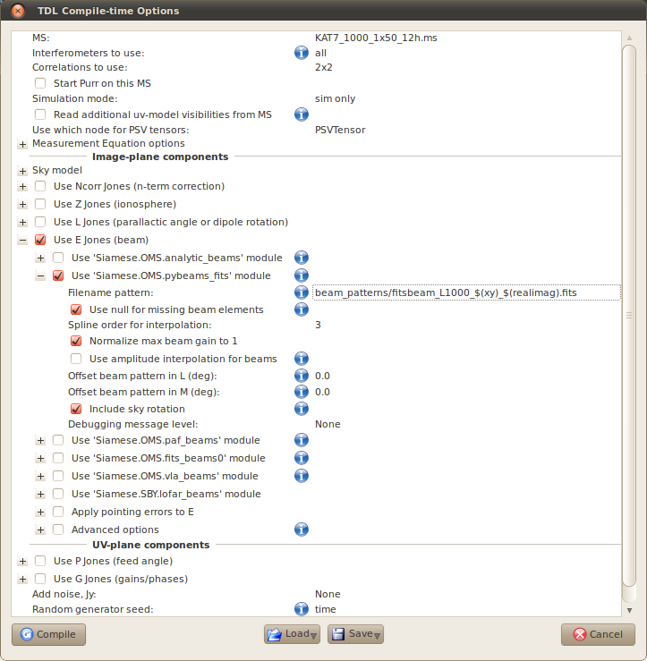
Now let's apply our simulated beam patterns to the simulation. Bring up the compile time options again and expand the 'Use E Jones (beam)' submenu. Check the "Use 'Siamese.OMS.pybeams_fits' module" option. Hovering the mouse pointer over the little 'i' information icons in the browser is always useful, and in the case of the 'Filename pattern' of this module, particularly so.
The beam patterns are specified here, and MeqTrees will substitute certain parts of the filename string that you enter, allowing you to specify mutliple correlation product beams, and also real and imaginary components in only one parameter.
In our example we are using:
beam_patterns/fitsbeam_L1000_$(xy)_$(realimag).fits
assuming the beam patterns are still in the beam_patterns folder. We're using the patterns appropriate for the 1000 MHz simulation (i.e. this MS). Instead of $(xy) when the simulation compiles, MeqTrees will loop over 'xx', 'xy', 'yx' and 'yy' into the filename, and similarly instead of $(realimag) it will loop over 'real' and 'imag', thus utilising the appropriate beam pattern at the appropriate place.
A couple of other options here are also pretty important. We want to check 'Use null for missing beam elements', as you will recall we are not using cross polarization beams, so MeqTrees will just assume these have zero gains. I've also checked 'Normalize max beam gain to 1', which fixes the boresight beam gain to unity.
Finally, another important option: ensure that you have checked 'Include sky rotation'. This rotates the beam pattern on the sky as the observation progresses as is the case for a genuine observation with an alt-az mount.
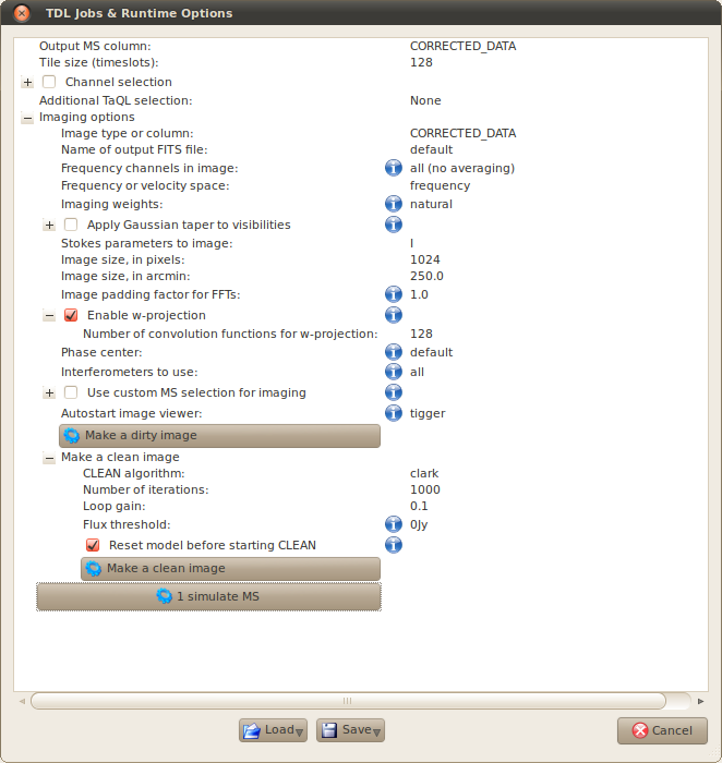
Click 'Compile', open a bookmark if you want, ensure we are writing to CORRECTED_DATA and then click '1 simulate MS' to write the visibilities.
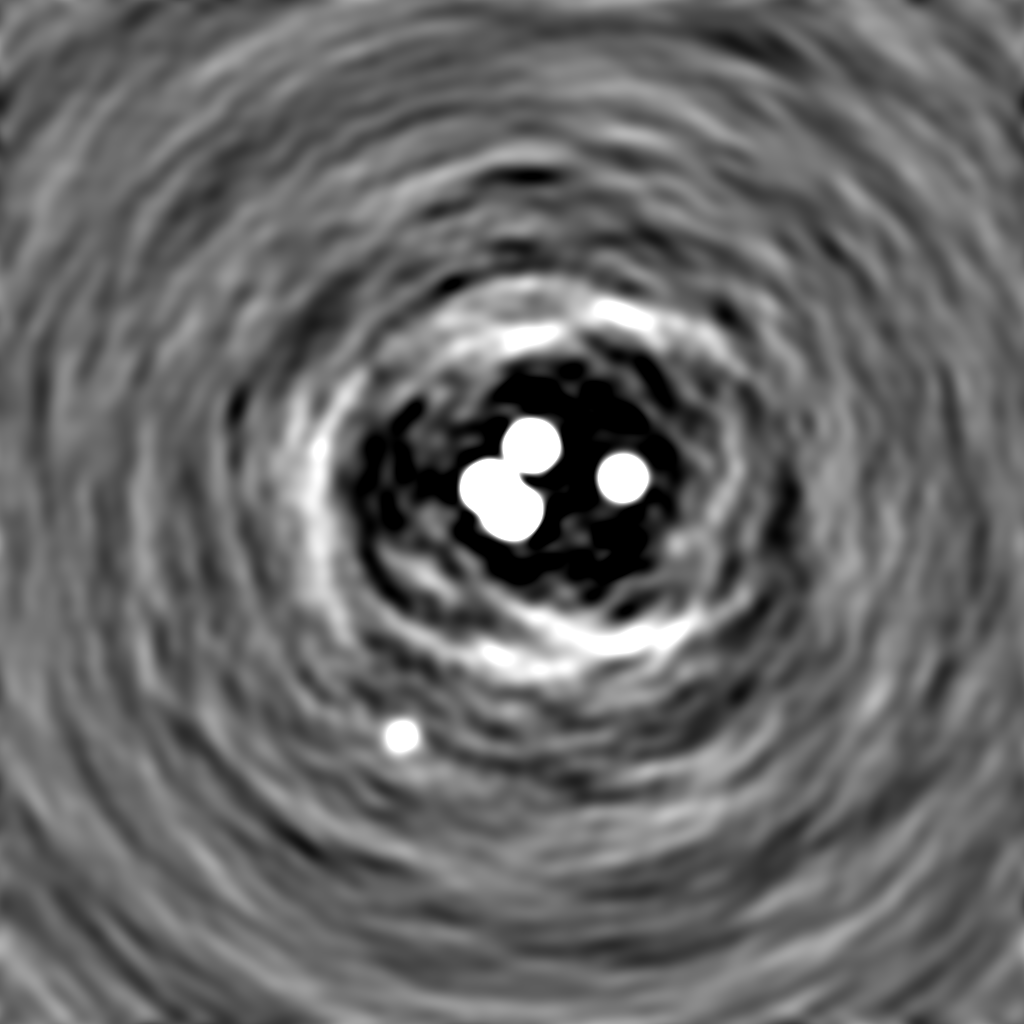
Once this has been successful, pop up the 'TDL Exec' menu again and make a cleaned image. The reason we're cleaning these images is that for sources that get attenuated away from the beam centre, you may find them being rendered invisible due to the strength of the sidelobes associated with the brightest sources in the field. You should be able to see, even in the thumbnail below, the attenuation effects of the beam.
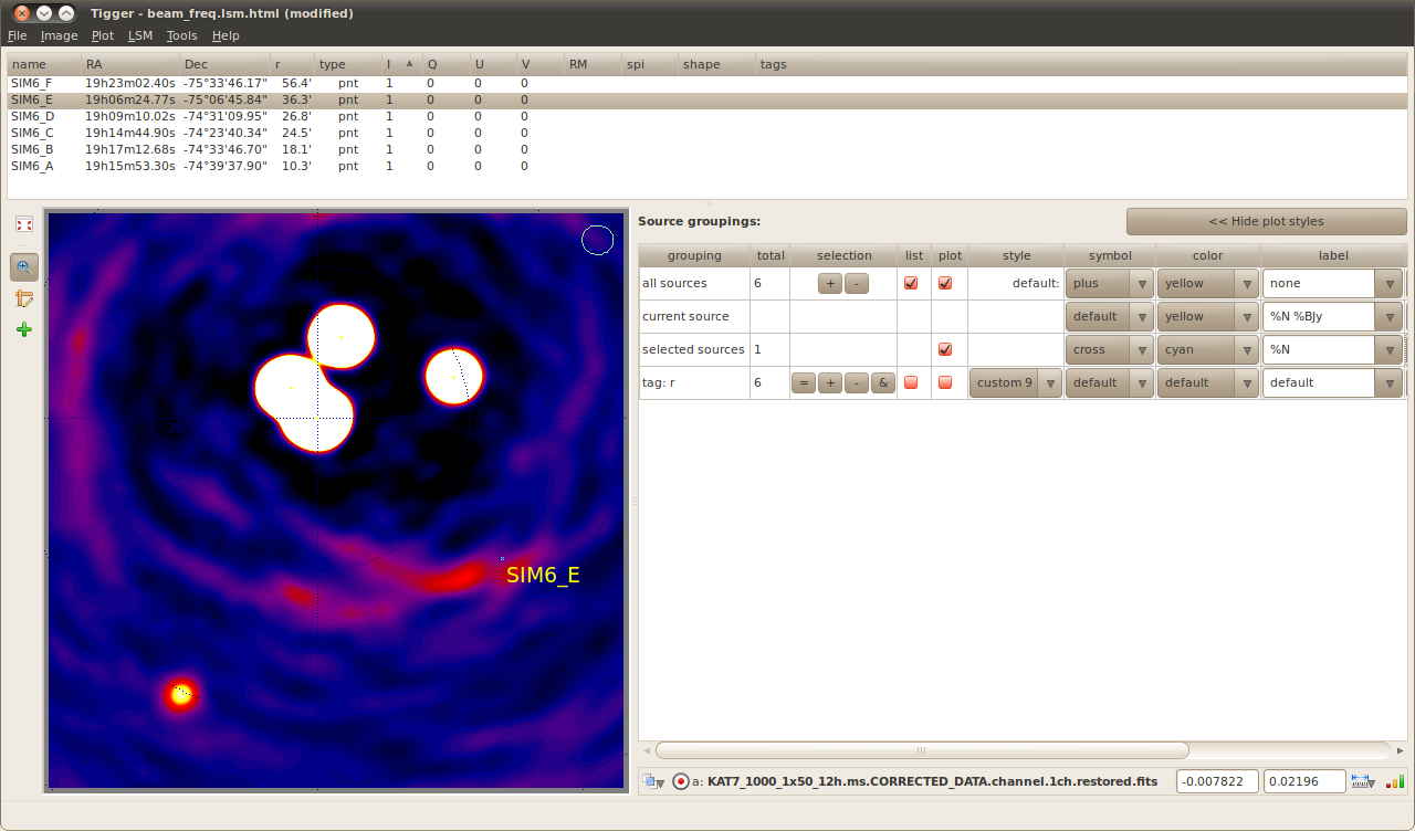
In fact, it looks like source SIM6_E has completely vanished. Did we forget something? I don't think we did, so where has it gone?
You can load the FITS image up together with the sky model to examine its precise position as I have done in the screenshot below. If you saved the intrinsic FITS image under a different name then you can also play around with image differencing.
Anyway, that's one frequency channel. One final thing before we deal with the other five is to open the 'TDL Exec' menu (or the compile time options) and save the profile under 'source_colourization_apparent'. Again a standalone .tdl.conf profile for this simulation is provided in the data products below.
 |
||||||||||||||||
 |
||||||||||||||||
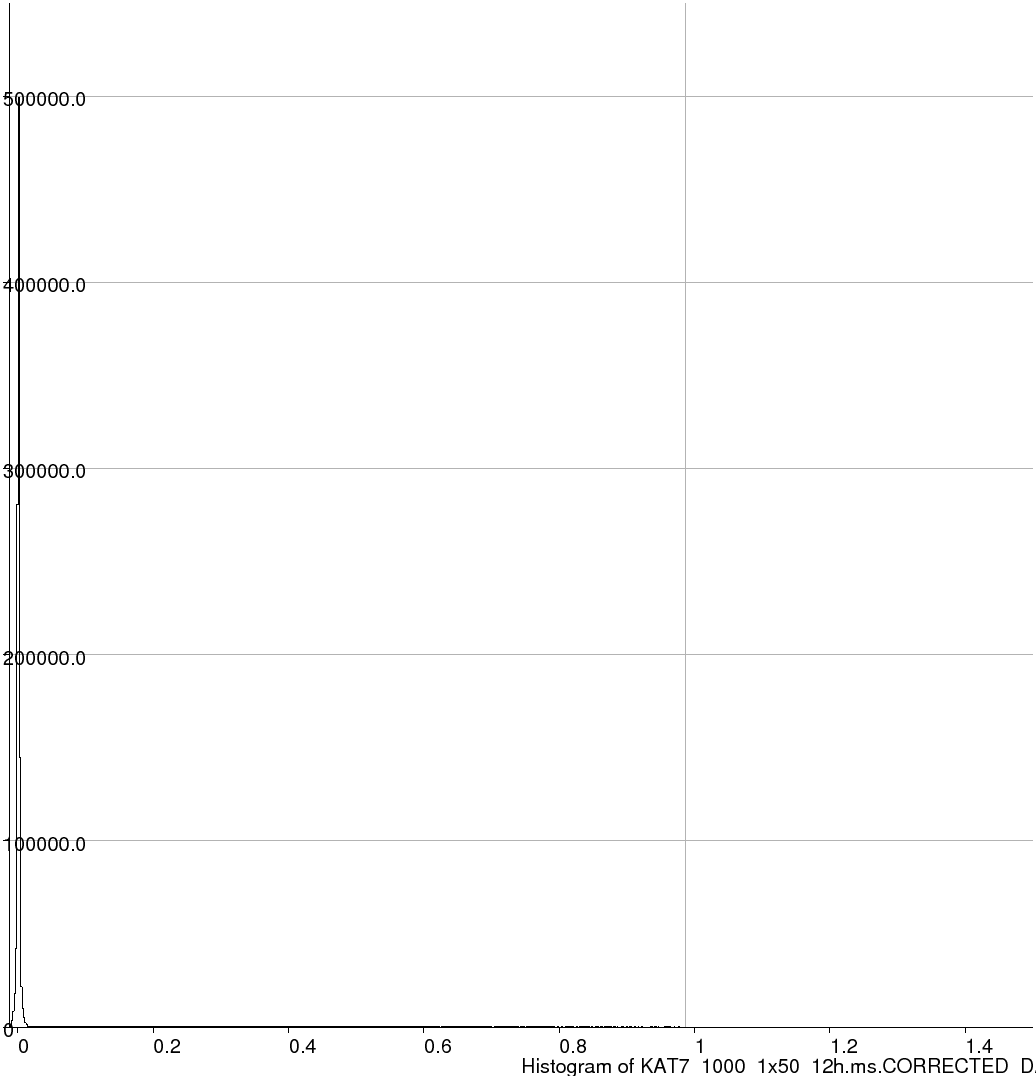
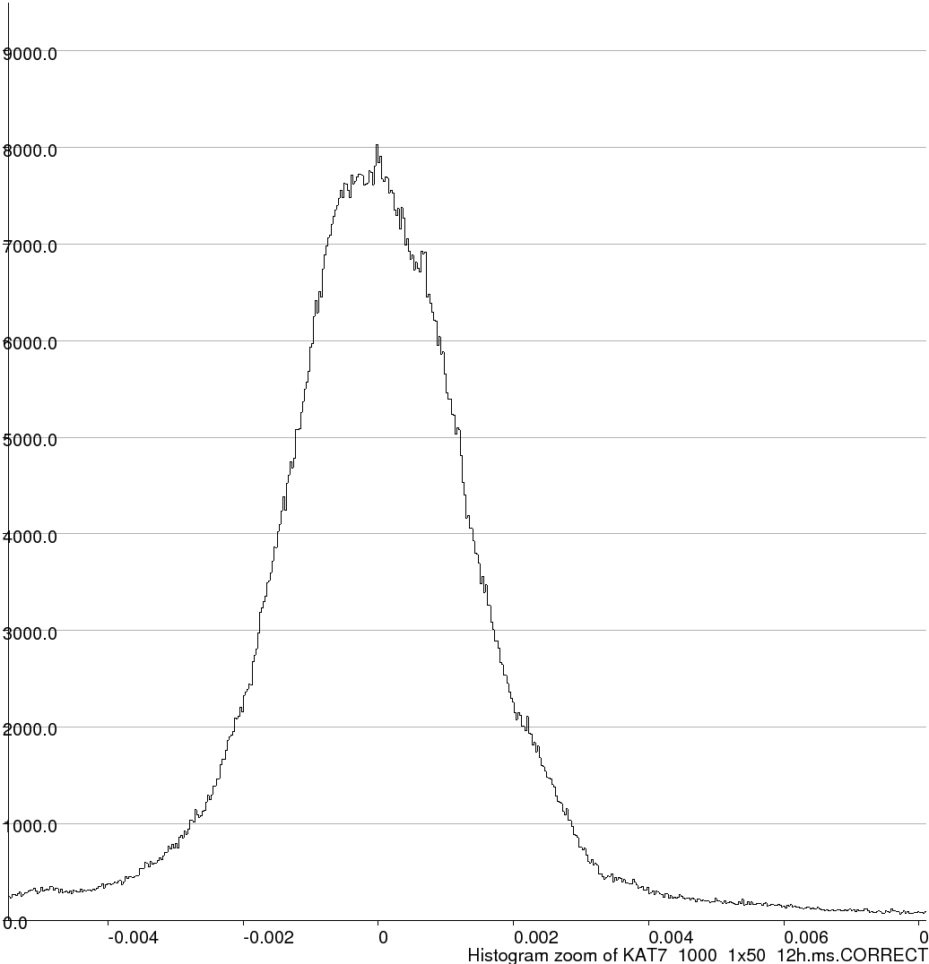
KAT7_1000_1x50_12h.ms.CORRECTED_DATA.channel.1ch.restored.fits (header) | ||||||||||||||||
|
|
|||||||||||||||
 |
||||||||||||||||